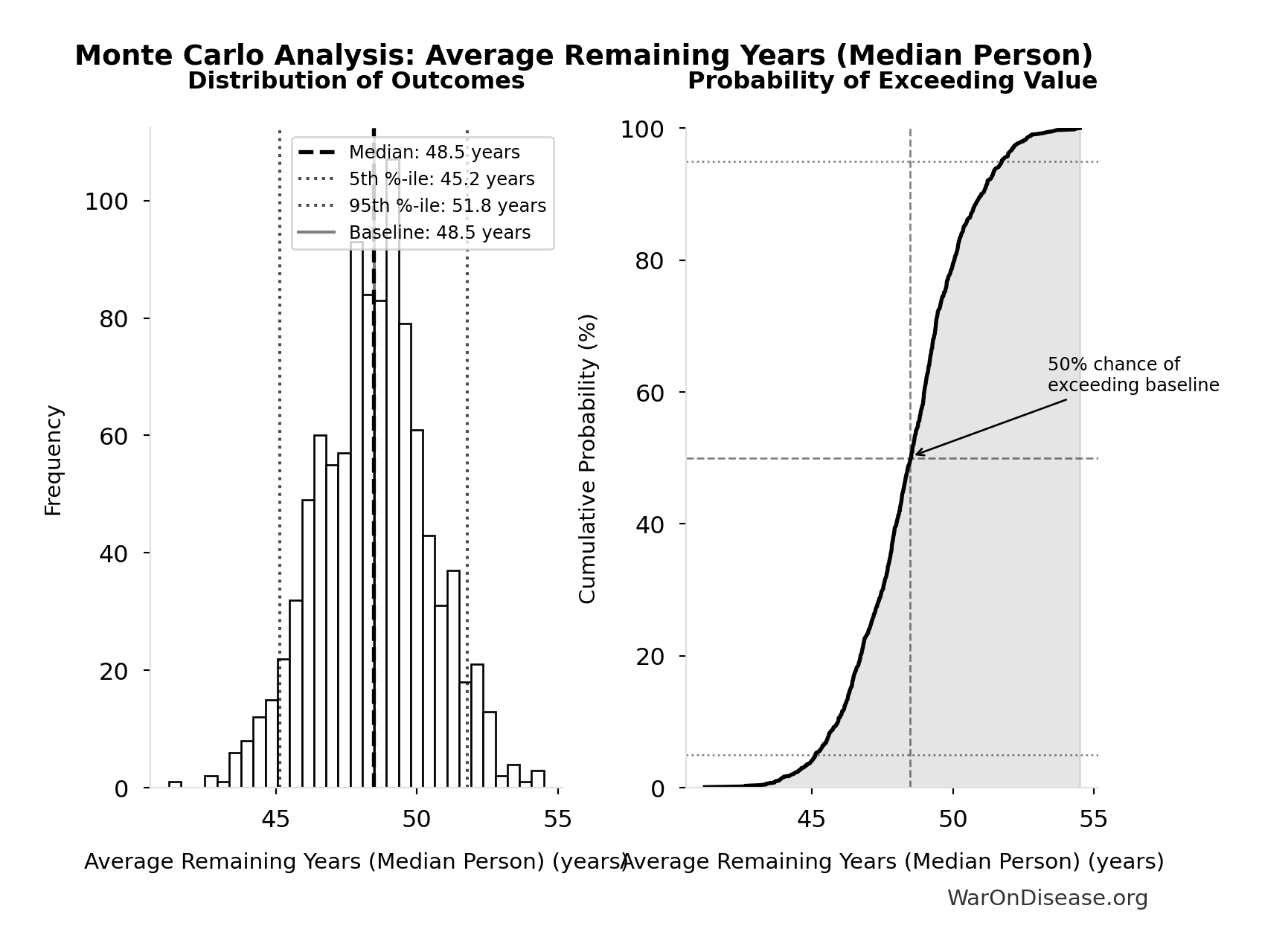
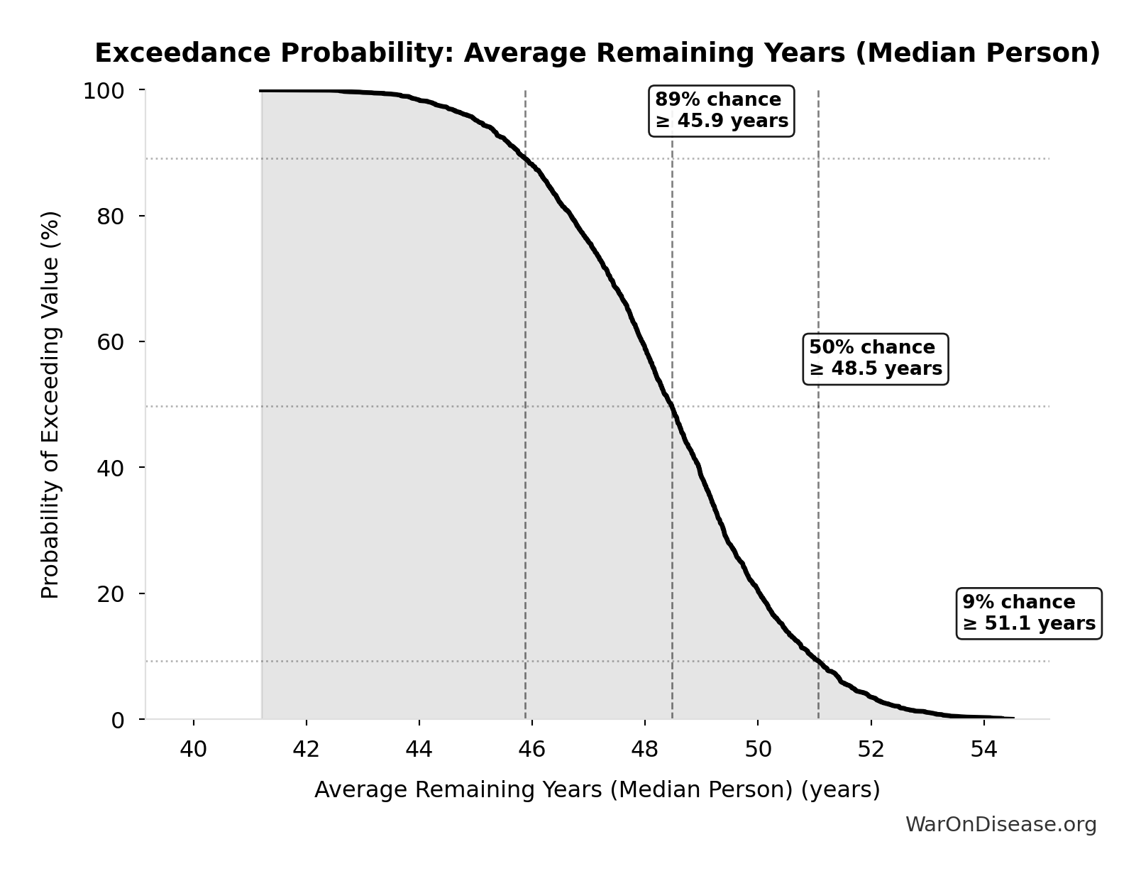
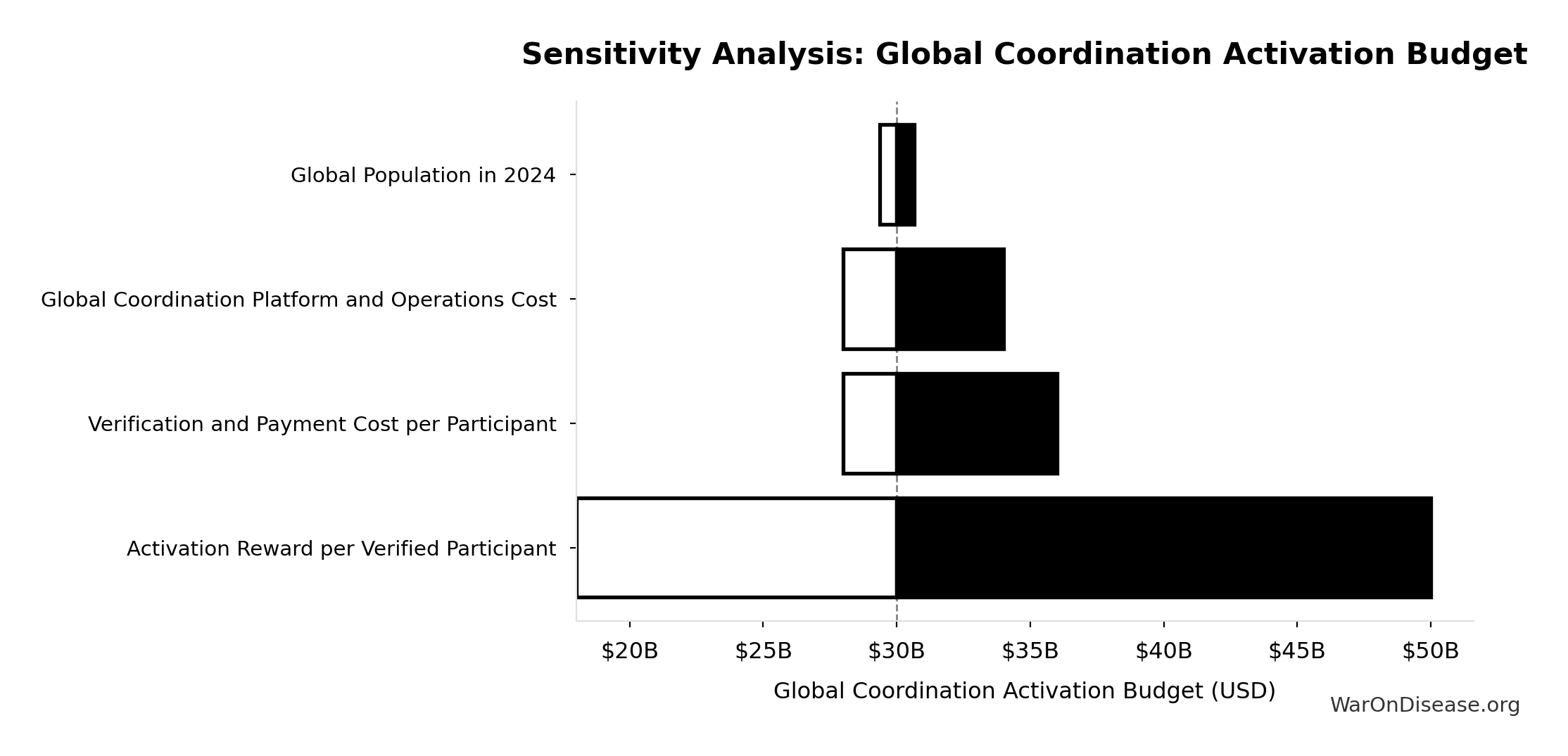
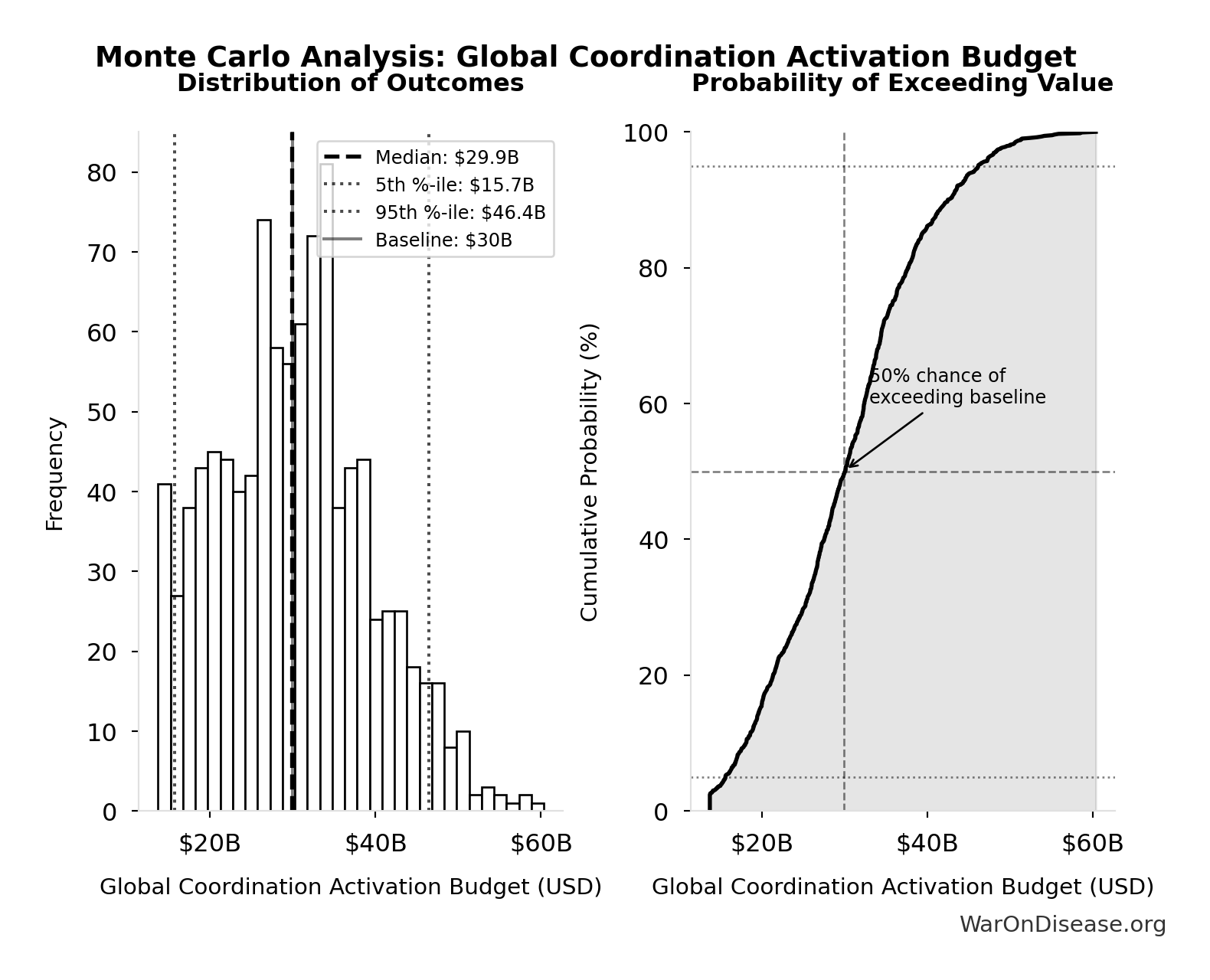
Methodology, Parameters, and Calculations
health economics methodology, clinical trial cost analysis, medical research ROI, cost-benefit analysis healthcare, sensitivity analysis, Monte Carlo simulation, DALY calculation, pragmatic clinical trials
Overview
This appendix documents all 526 parameters used in the analysis, organized by type:
- External sources (peer-reviewed): 171
- Calculated values: 250
- Core definitions: 105
Calculated Values
Parameters derived from mathematical formulas and economic models.
Engagement Rate: 10%
Probability someone engages with the idea (1 - dismissal rate)
Inputs:
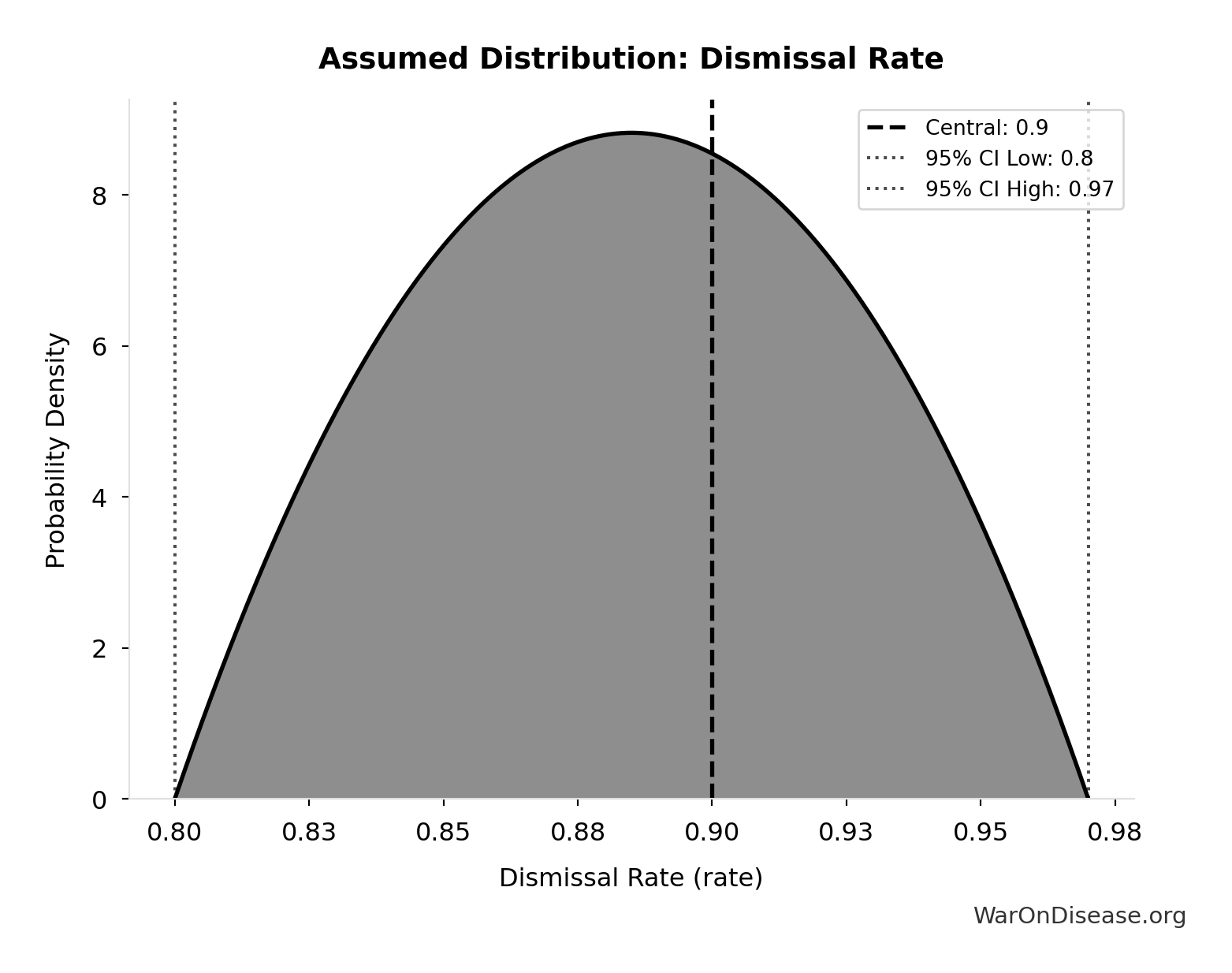
- Dismissal Rate: 90% (95% CI: 80% - 97%)
\[ P_{engage} = 1 - P_{dismiss} = 1 - 90\% = 10\% \]
✓ High confidence
Sensitivity Analysis
Sensitivity Indices for Engagement Rate
Regression-based sensitivity showing which inputs explain the most variance in the output.
| Input Parameter | Sensitivity Coefficient | Interpretation |
|---|---|---|
| Dismissal Rate (rate) | -1.0000 | Strong driver |
Interpretation: Standardized coefficients show the change in output (in SD units) per 1 SD change in input. Values near ±1 indicate strong influence; values exceeding ±1 may occur with correlated inputs.
Monte Carlo Distribution
Simulation Results Summary: Engagement Rate
| Statistic | Value |
|---|---|
| Baseline (deterministic) | 10% |
| Mean (expected value) | 9.97% |
| Median (50th percentile) | 9.46% |
| Standard Deviation | 4.18% |
| 90% Range (5th-95th percentile) | [3.91%, 18.1%] |
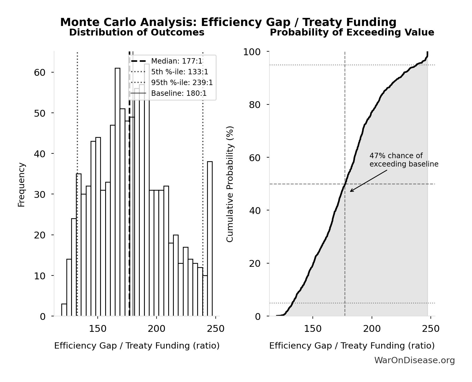
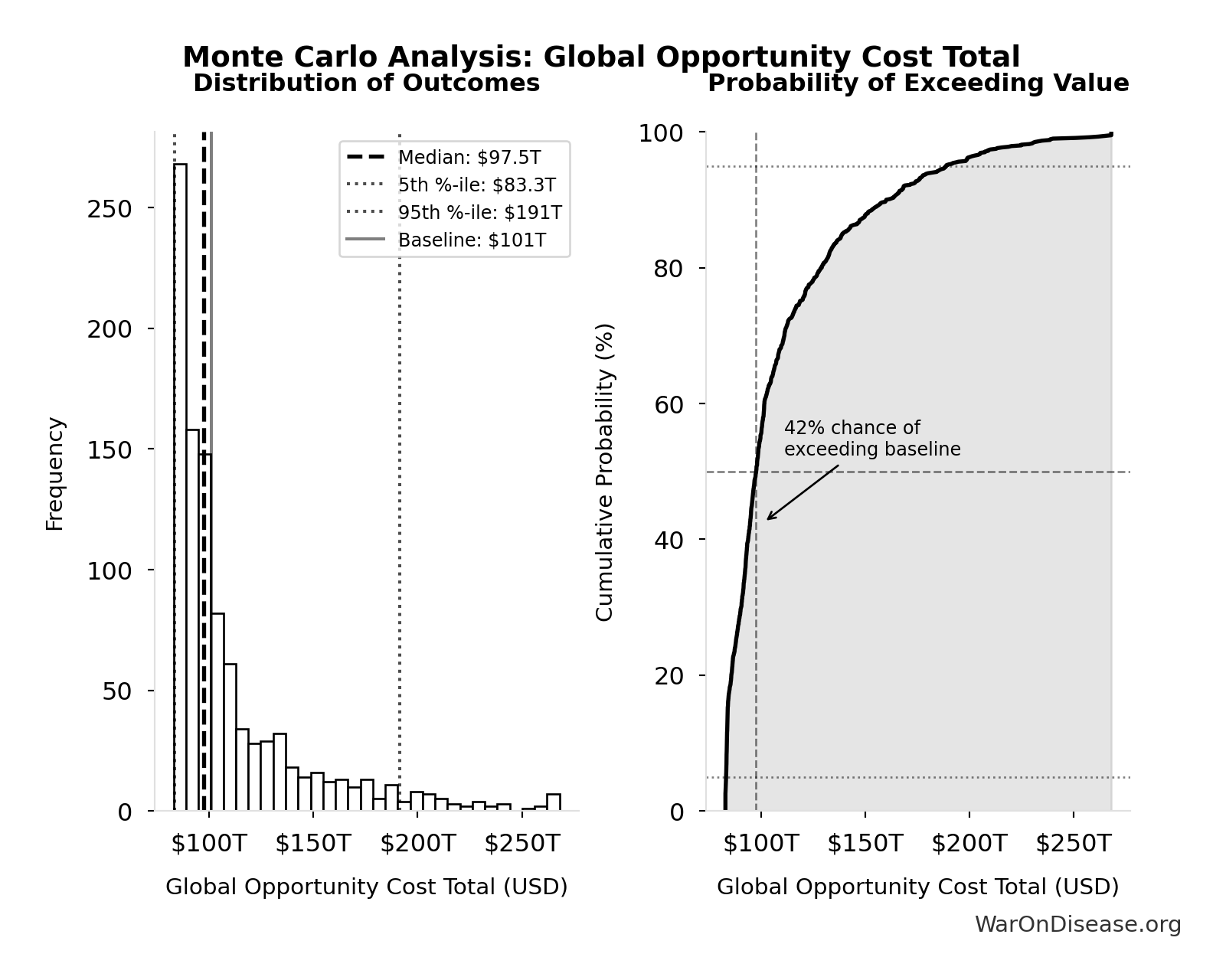
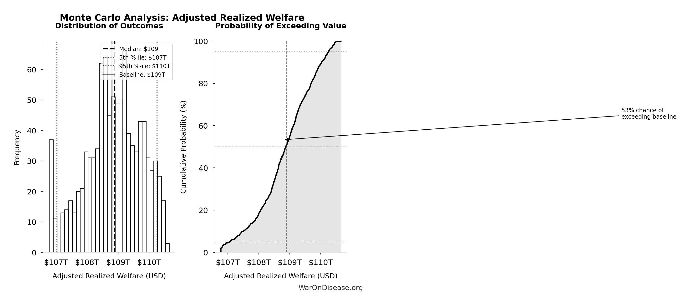
The histogram shows the distribution of Engagement Rate across 10,000 Monte Carlo simulations. The CDF (right) shows the probability of the outcome exceeding any given value, which is useful for risk assessment.
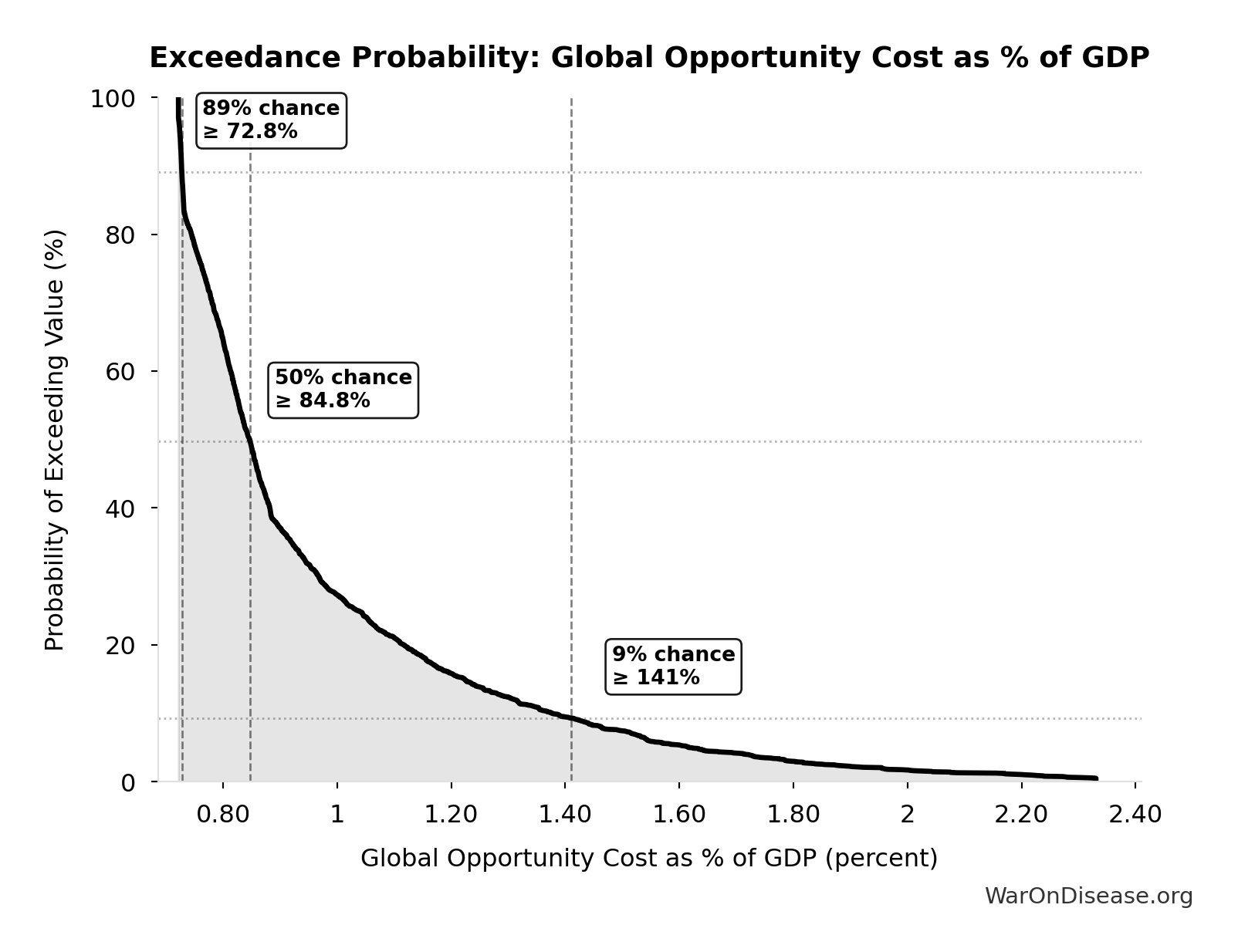
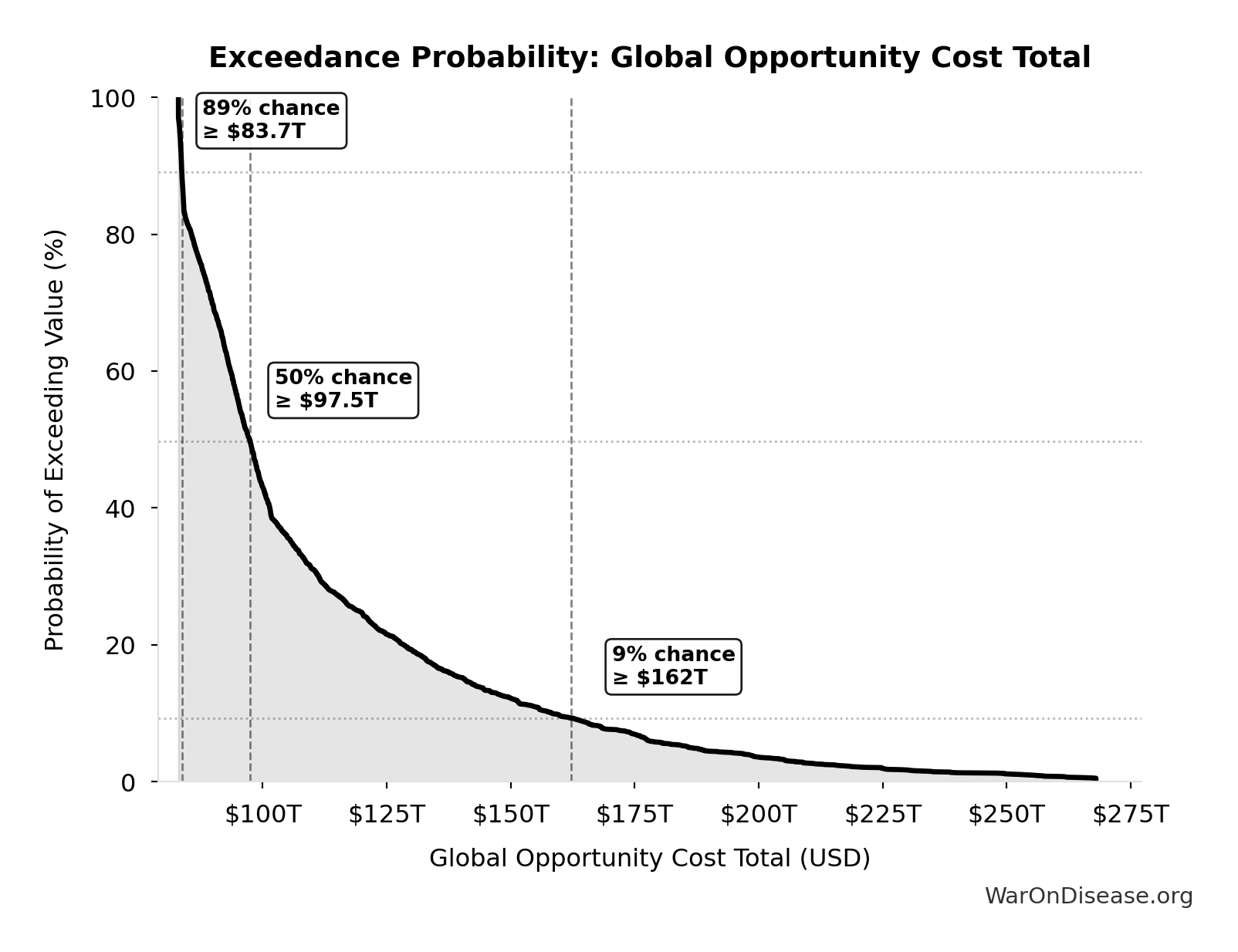
Exceedance Probability
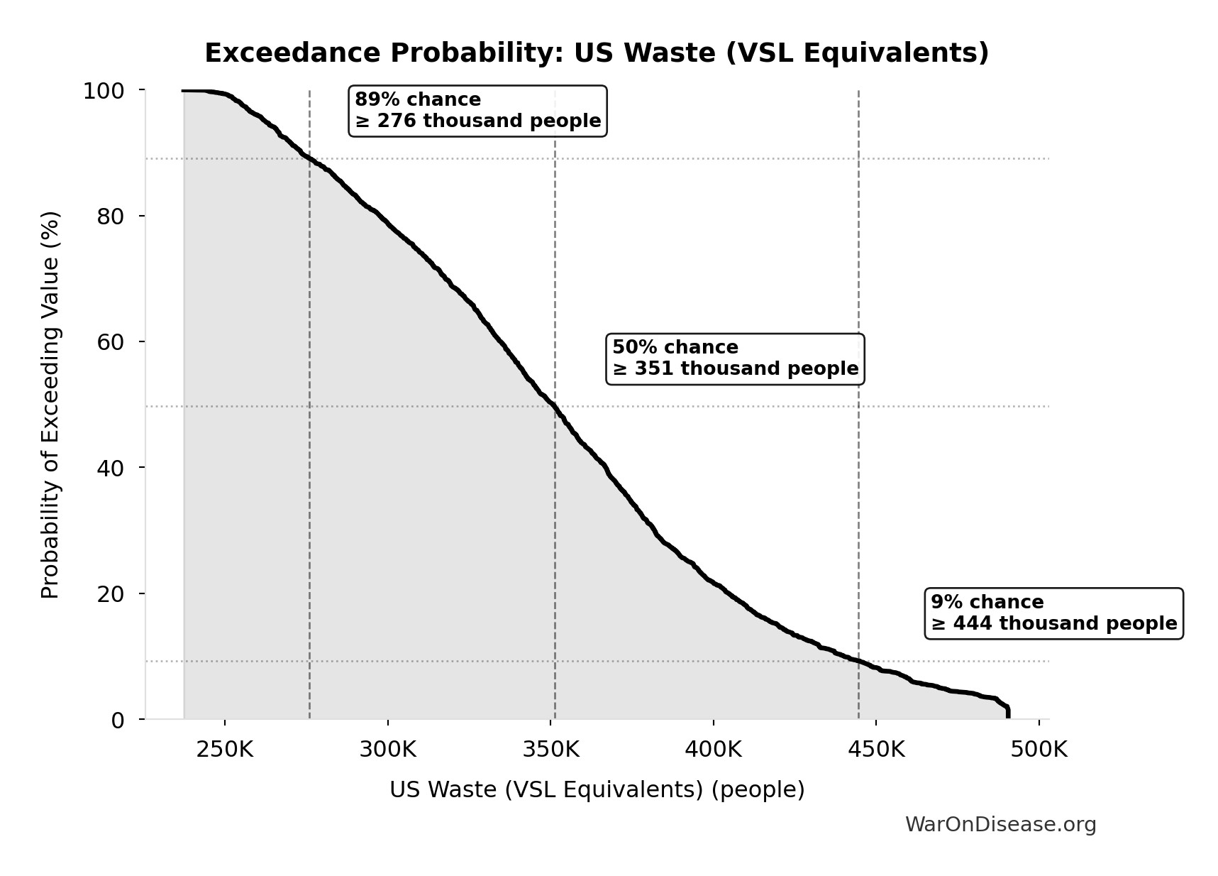
This exceedance probability chart shows the likelihood that Engagement Rate will exceed any given threshold. Higher curves indicate more favorable outcomes with greater certainty.
Expected Engaged Implementers: 3.48 people
Expected number of implementers who engage (orbit reached x engagement rate x implementer count)
Inputs:
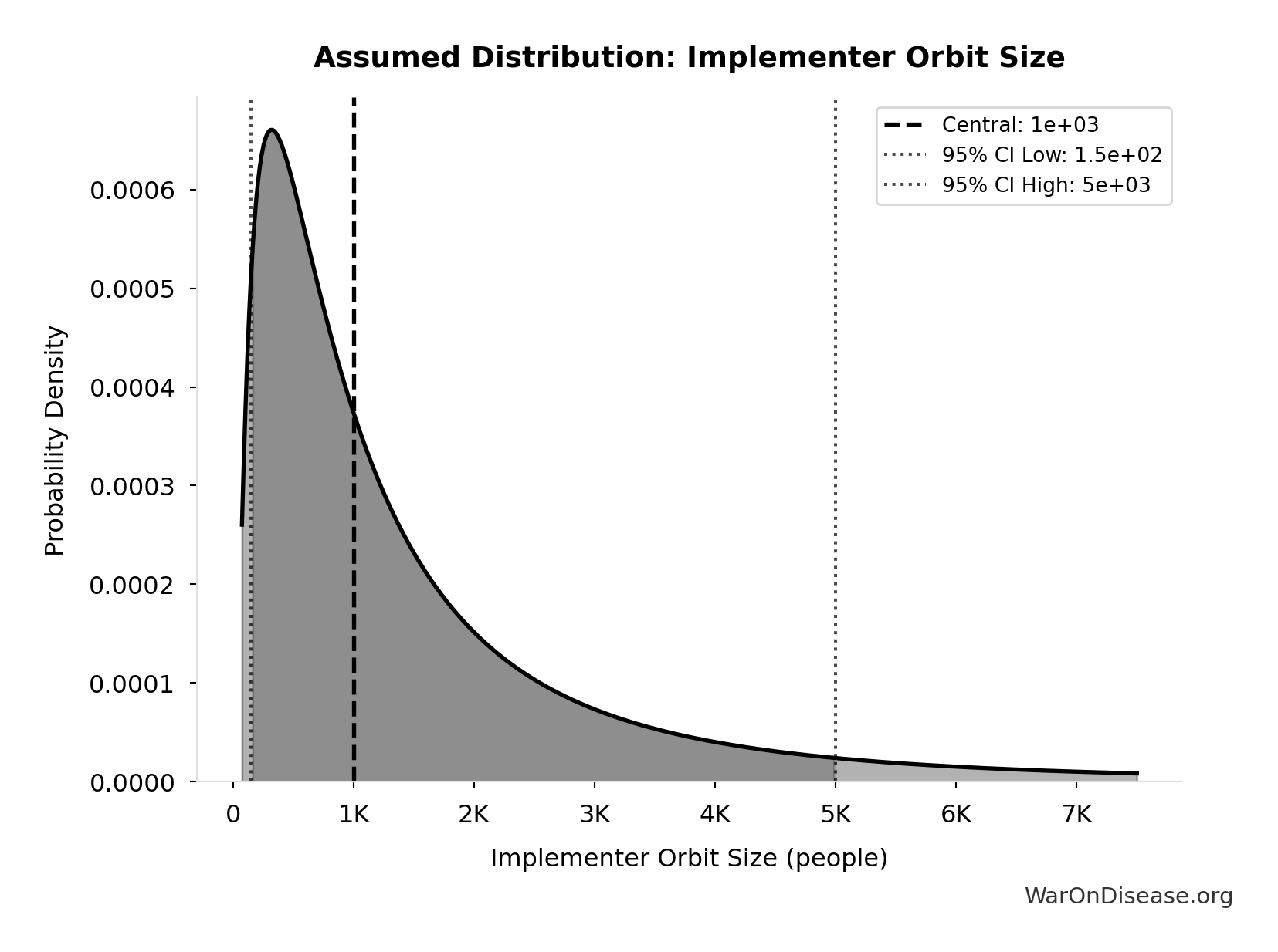
- Implementer Orbit Size: 1 thousand people (95% CI: 150 people - 5 thousand people)
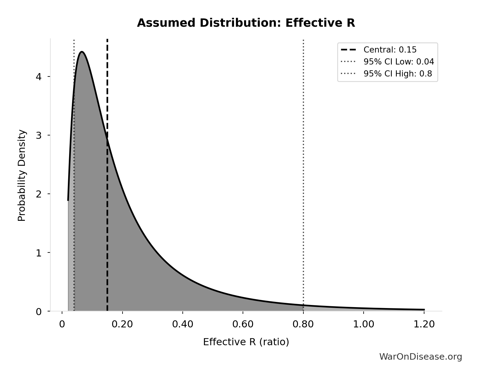
- Effective R: 0.15:1 (95% CI: 0.04:1 - 0.8:1)
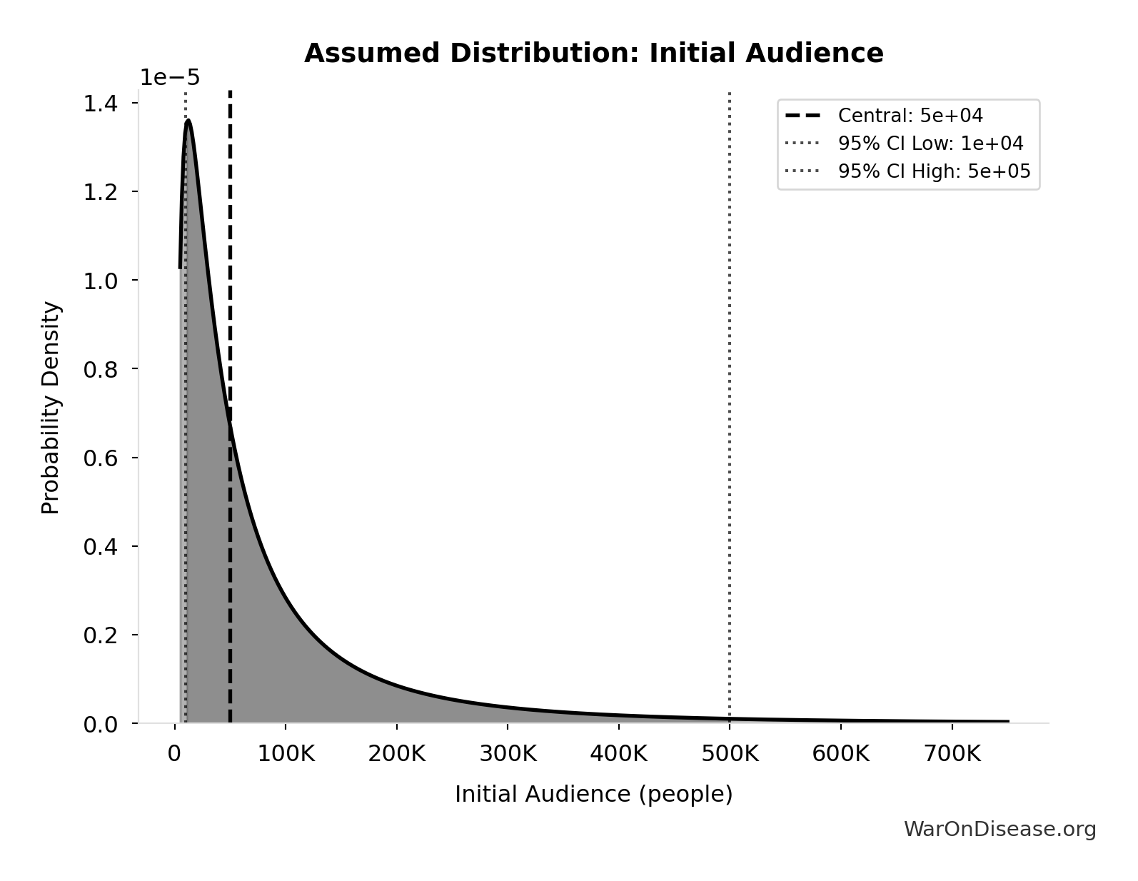
- Initial Audience: 50 thousand people (95% CI: 10 thousand people - 500 thousand people)
- Engagement Rate 🔢: 10%
- Potential Implementers 🔢: 2.98 thousand people
\[ E[N_{engaged}] = P_{reach} \times P_{engage} \times N_{impl} \]
✓ High confidence
Sensitivity Analysis
Sensitivity Indices for Expected Engaged Implementers
Regression-based sensitivity showing which inputs explain the most variance in the output.
| Input Parameter | Sensitivity Coefficient | Interpretation |
|---|---|---|
| Initial Audience (people) | 1.7614 | Strong driver |
| Effective R (ratio) | -1.5003 | Strong driver |
| Implementer Orbit Size (people) | 0.6074 | Strong driver |
| Engagement Rate (rate) | 0.1146 | Weak driver |
Interpretation: Standardized coefficients show the change in output (in SD units) per 1 SD change in input. Values near ±1 indicate strong influence; values exceeding ±1 may occur with correlated inputs.
Monte Carlo Distribution
Simulation Results Summary: Expected Engaged Implementers
| Statistic | Value |
|---|---|
| Baseline (deterministic) | 3.48 |
| Mean (expected value) | 10.8 |
| Median (50th percentile) | 0.668 |
| Standard Deviation | 37.3 |
| 90% Range (5th-95th percentile) | [0.0736, 53.7] |
The histogram shows the distribution of Expected Engaged Implementers across 10,000 Monte Carlo simulations. The CDF (right) shows the probability of the outcome exceeding any given value, which is useful for risk assessment.
Exceedance Probability
This exceedance probability chart shows the likelihood that Expected Engaged Implementers will exceed any given threshold. Higher curves indicate more favorable outcomes with greater certainty.
Potential Implementers: 2.98 thousand people
Total potential implementers (billionaires + world leaders)
Inputs:
- Global Billionaire Count 📊: 2.78 thousand people
- World Leader Count: 195 countries
\[ \begin{gathered} N_{impl} \\ = N_{billionaire} + N_{leader} \\ = 2{,}780 + 195 \\ = 2{,}980 \end{gathered} \]
✓ High confidence
P(At Least One Engages): 96.9%
Probability at least one implementer engages (information diffusion only; dominant strategy proof handles action)
Inputs:
- P(No Implementer Engages) 🔢: 3.08%
\[ P_{reach} = 1 - P_{none} = 1 - 3.08\% = 96.9\% \] where: \[ \begin{gathered} P_{none} \\ = \left(1 - P_{reach} \cdot P_{engage}\right)^{N_{impl}} \end{gathered} \] where: \[ P_{engage} = 1 - P_{dismiss} = 1 - 90\% = 10\% \] where: \[ \begin{gathered} N_{impl} \\ = N_{billionaire} + N_{leader} \\ = 2{,}780 + 195 \\ = 2{,}980 \end{gathered} \] ✓ High confidence
Sensitivity Analysis
Sensitivity Indices for P(At Least One Engages)
Regression-based sensitivity showing which inputs explain the most variance in the output.
| Input Parameter | Sensitivity Coefficient | Interpretation |
|---|---|---|
| P(No Implementer Engages) (rate) | -1.0000 | Strong driver |
Interpretation: Standardized coefficients show the change in output (in SD units) per 1 SD change in input. Values near ±1 indicate strong influence; values exceeding ±1 may occur with correlated inputs.
Monte Carlo Distribution
Simulation Results Summary: P(At Least One Engages)
| Statistic | Value |
|---|---|
| Baseline (deterministic) | 96.9% |
| Mean (expected value) | 54% |
| Median (50th percentile) | 48.7% |
| Standard Deviation | 36.6% |
| 90% Range (5th-95th percentile) | [7.09%, 100%] |
The histogram shows the distribution of P(At Least One Engages) across 10,000 Monte Carlo simulations. The CDF (right) shows the probability of the outcome exceeding any given value, which is useful for risk assessment.
Exceedance Probability
This exceedance probability chart shows the likelihood that P(At Least One Engages) will exceed any given threshold. Higher curves indicate more favorable outcomes with greater certainty.
Implementer Orbit Reach Probability: 1.17%
Probability a given implementer’s information orbit is reached by the content cascade
Inputs:
- Implementer Orbit Size: 1 thousand people (95% CI: 150 people - 5 thousand people)
- Effective R: 0.15:1 (95% CI: 0.04:1 - 0.8:1)
- Initial Audience: 50 thousand people (95% CI: 10 thousand people - 500 thousand people)
\[ \begin{gathered} P_{reach} \\ = 1 - \left(1 - \frac{O_{impl}}{N}\right)^{N_0 \cdot \sum_{i=0}^{3} R_{eff}^i} \end{gathered} \]
✓ High confidence
Sensitivity Analysis
Sensitivity Indices for Implementer Orbit Reach Probability
Regression-based sensitivity showing which inputs explain the most variance in the output.
| Input Parameter | Sensitivity Coefficient | Interpretation |
|---|---|---|
| Initial Audience (people) | 1.8982 | Strong driver |
| Effective R (ratio) | -1.5989 | Strong driver |
| Implementer Orbit Size (people) | 0.6433 | Strong driver |
Interpretation: Standardized coefficients show the change in output (in SD units) per 1 SD change in input. Values near ±1 indicate strong influence; values exceeding ±1 may occur with correlated inputs.
Monte Carlo Distribution
Simulation Results Summary: Implementer Orbit Reach Probability
| Statistic | Value |
|---|---|
| Baseline (deterministic) | 1.17% |
| Mean (expected value) | 3.62% |
| Median (50th percentile) | 0.248% |
| Standard Deviation | 11.5% |
| 90% Range (5th-95th percentile) | [0.0312%, 18.6%] |
The histogram shows the distribution of Implementer Orbit Reach Probability across 10,000 Monte Carlo simulations. The CDF (right) shows the probability of the outcome exceeding any given value, which is useful for risk assessment.
Exceedance Probability
This exceedance probability chart shows the likelihood that Implementer Orbit Reach Probability will exceed any given threshold. Higher curves indicate more favorable outcomes with greater certainty.
P(No Implementer Engages): 3.08%
Probability that NO implementer engages (all orbits missed or all dismiss)
Inputs:
- Implementer Orbit Size: 1 thousand people (95% CI: 150 people - 5 thousand people)
- Effective R: 0.15:1 (95% CI: 0.04:1 - 0.8:1)
- Initial Audience: 50 thousand people (95% CI: 10 thousand people - 500 thousand people)
- Engagement Rate 🔢: 10%
- Potential Implementers 🔢: 2.98 thousand people
\[ \begin{gathered} P_{none} \\ = \left(1 - P_{reach} \cdot P_{engage}\right)^{N_{impl}} \end{gathered} \]
✓ High confidence
Sensitivity Analysis
Sensitivity Indices for P(No Implementer Engages)
Regression-based sensitivity showing which inputs explain the most variance in the output.
| Input Parameter | Sensitivity Coefficient | Interpretation |
|---|---|---|
| Implementer Orbit Size (people) | -3.6645 | Strong driver |
| Effective R (ratio) | 1.5260 | Strong driver |
| Initial Audience (people) | 1.4706 | Strong driver |
| Engagement Rate (rate) | -0.1870 | Weak driver |
Interpretation: Standardized coefficients show the change in output (in SD units) per 1 SD change in input. Values near ±1 indicate strong influence; values exceeding ±1 may occur with correlated inputs.
Monte Carlo Distribution
Simulation Results Summary: P(No Implementer Engages)
| Statistic | Value |
|---|---|
| Baseline (deterministic) | 3.08% |
| Mean (expected value) | 46% |
| Median (50th percentile) | 51.3% |
| Standard Deviation | 36.6% |
| 90% Range (5th-95th percentile) | [2.79e-22%, 92.9%] |
The histogram shows the distribution of P(No Implementer Engages) across 10,000 Monte Carlo simulations. The CDF (right) shows the probability of the outcome exceeding any given value, which is useful for risk assessment.
Exceedance Probability
This exceedance probability chart shows the likelihood that P(No Implementer Engages) will exceed any given threshold. Higher curves indicate more favorable outcomes with greater certainty.
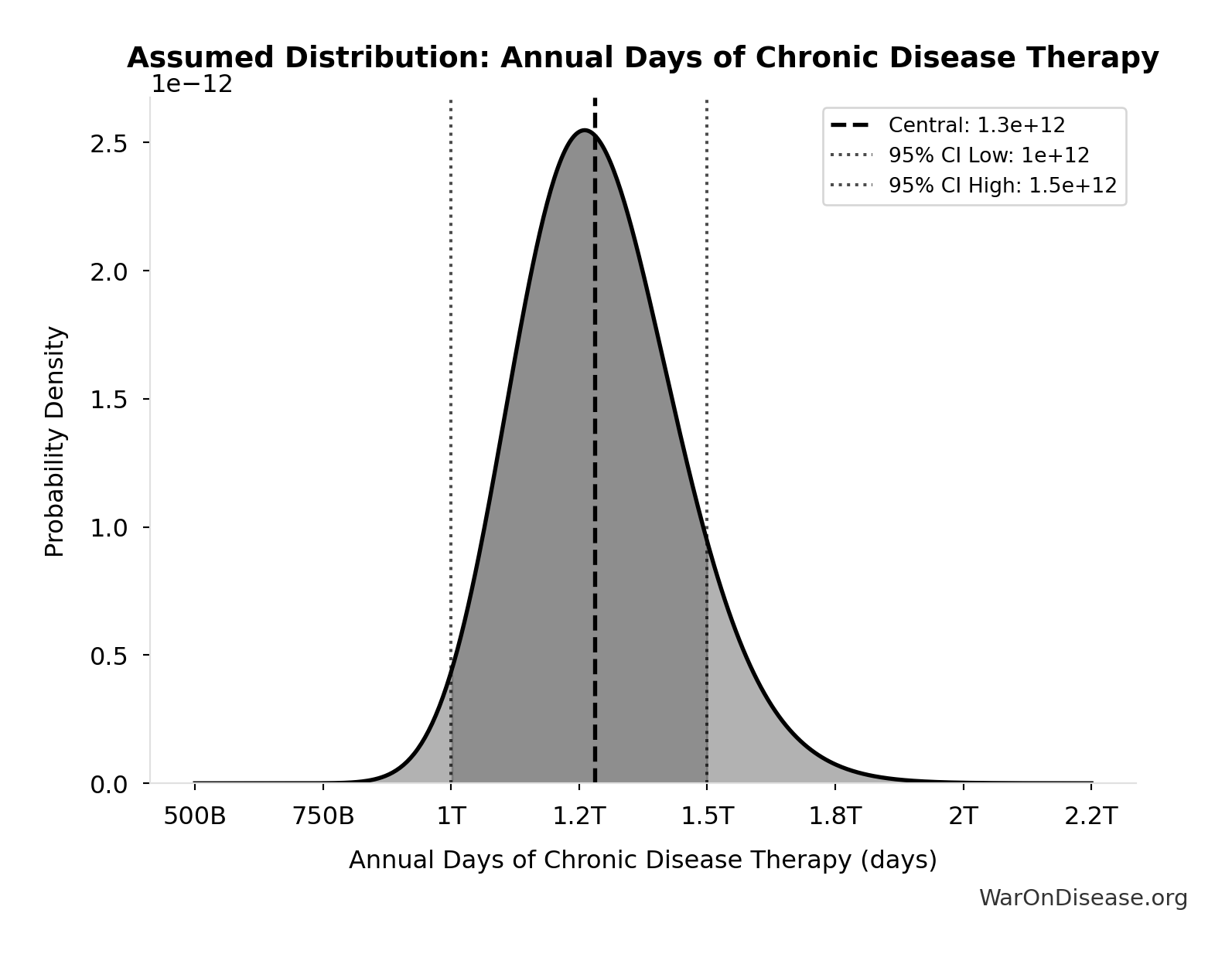
Annual Chronic Disease Patients Treated: 982 million people
Estimated unique patients receiving chronic disease treatment annually. Derived from IQVIA days of therapy (1.28T) divided by 365 days divided by 2.5 average medications per patient times 70% post-1962 drugs.
Inputs:
- Annual Days of Chronic Disease Therapy 📊: 1.28 trillion days (95% CI: 1 trillion days - 1.5 trillion days)
\[ \begin{gathered} N_{treated} \\ = DOT_{chronic} \times 0.000767 \\ = 1.28T \times 0.000767 \\ = 982M \end{gathered} \]
Methodology:45
? Low confidence
Sensitivity Analysis
Sensitivity Indices for Annual Chronic Disease Patients Treated
Regression-based sensitivity showing which inputs explain the most variance in the output.
| Input Parameter | Sensitivity Coefficient | Interpretation |
|---|---|---|
| Annual Days of Chronic Disease Therapy (days) | 1.0000 | Strong driver |
Interpretation: Standardized coefficients show the change in output (in SD units) per 1 SD change in input. Values near ±1 indicate strong influence; values exceeding ±1 may occur with correlated inputs.
Monte Carlo Distribution
Simulation Results Summary: Annual Chronic Disease Patients Treated
| Statistic | Value |
|---|---|
| Baseline (deterministic) | 982 million |
| Mean (expected value) | 981 million |
| Median (50th percentile) | 976 million |
| Standard Deviation | 98.4 million |
| 90% Range (5th-95th percentile) | [827 million, 1.15 billion] |
The histogram shows the distribution of Annual Chronic Disease Patients Treated across 10,000 Monte Carlo simulations. The CDF (right) shows the probability of the outcome exceeding any given value, which is useful for risk assessment.
Exceedance Probability
This exceedance probability chart shows the likelihood that Annual Chronic Disease Patients Treated will exceed any given threshold. Higher curves indicate more favorable outcomes with greater certainty.
Combination Therapy Space: 45.1 billion combinations
Total combination therapy space (pairwise drug combinations × diseases). Standard in oncology, HIV, cardiology.
Inputs:
- Pairwise Drug Combinations 🔢: 45.1 million combinations
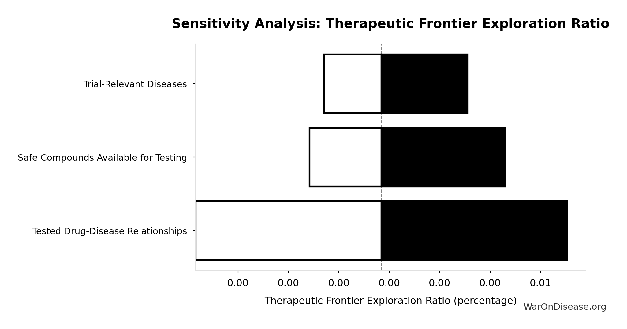
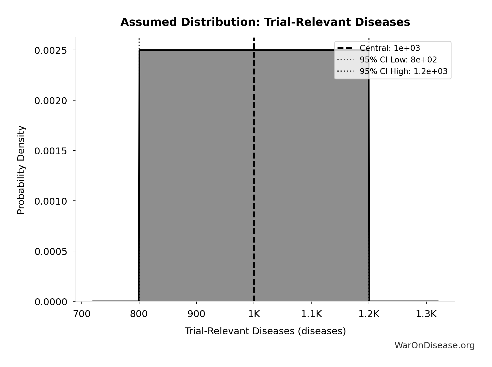
- Trial-Relevant Diseases: 1 thousand diseases (95% CI: 800 diseases - 1.2 thousand diseases)
\[ \begin{gathered} Space_{combo} \\ = N_{combo} \times N_{diseases,trial} \\ = 45.1M \times 1{,}000 \\ = 45.1B \end{gathered} \]
✓ High confidence
Sensitivity Analysis
Pairwise Drug Combinations: 45.1 million combinations
Unique pairwise drug combinations from known safe compounds (n choose 2)
Inputs:
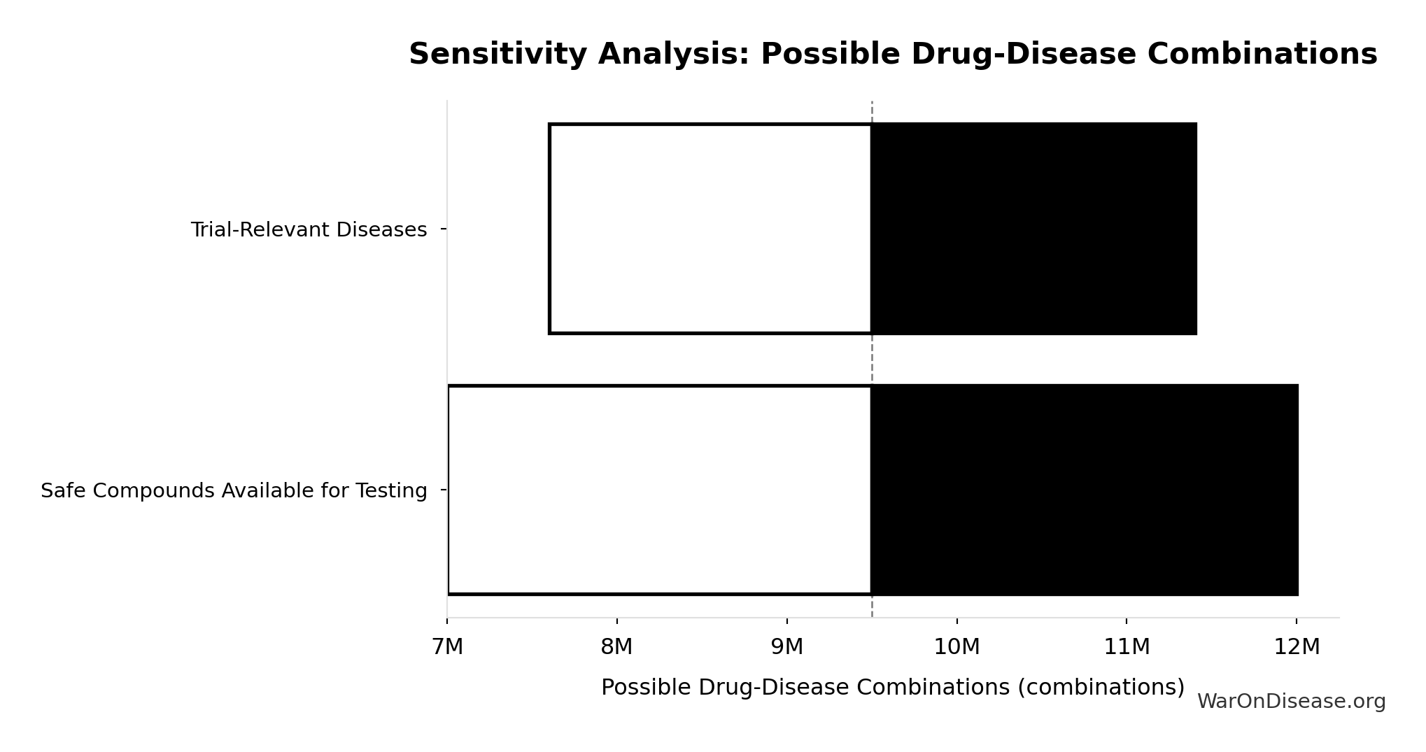
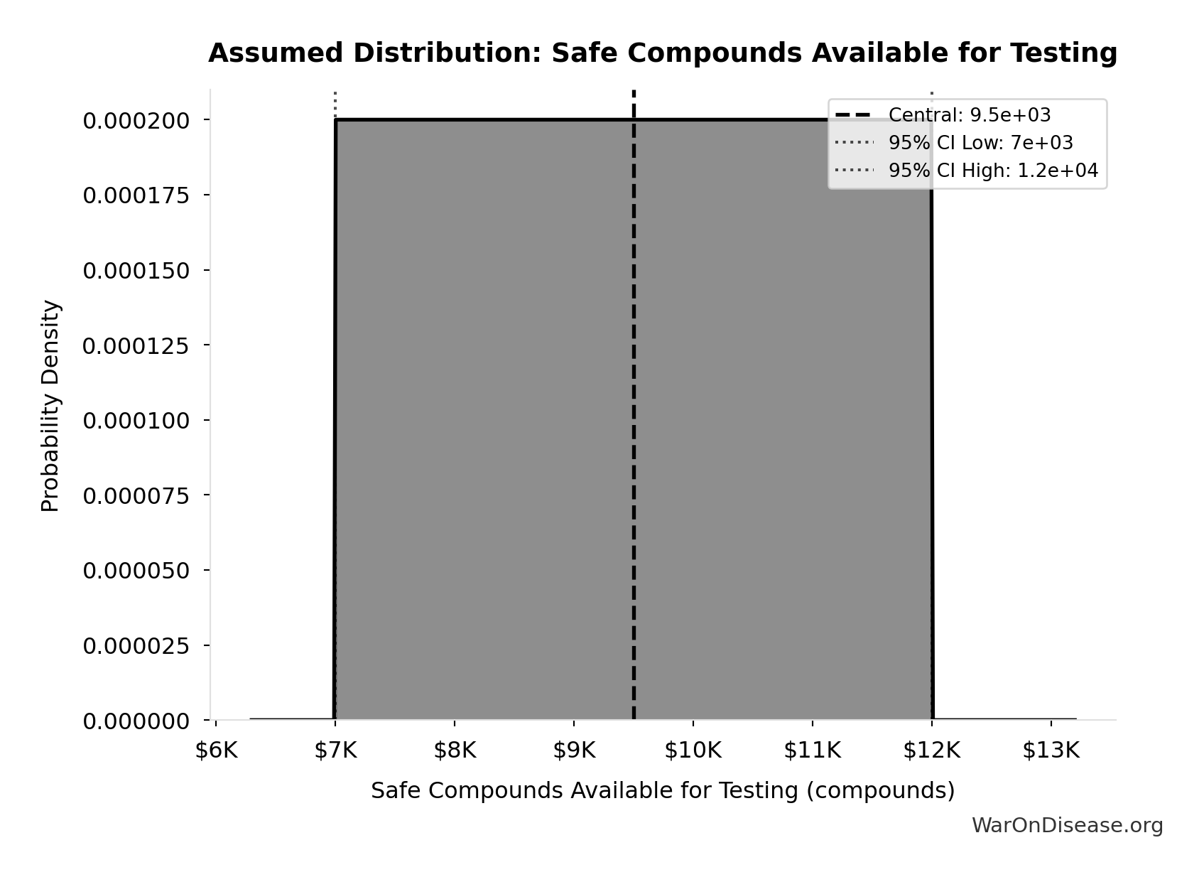
- Safe Compounds Available for Testing: 9.5 thousand compounds (95% CI: 7 thousand compounds - 12 thousand compounds)
Formula: SAFE_COMPOUNDS × (SAFE_COMPOUNDS - 1) ÷ 2
✓ High confidence
Sensitivity Analysis
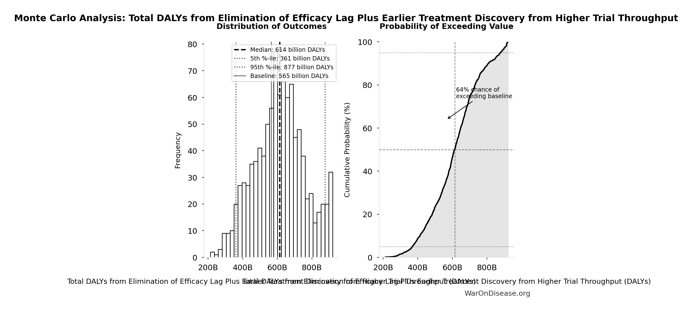
DALYs Averted per Percentage Point: 5.65 billion DALYs
DALYs averted per percentage point of implementation probability shift. One percent of total DALYs from eliminating trial capacity bottleneck and efficacy lag.
Inputs:
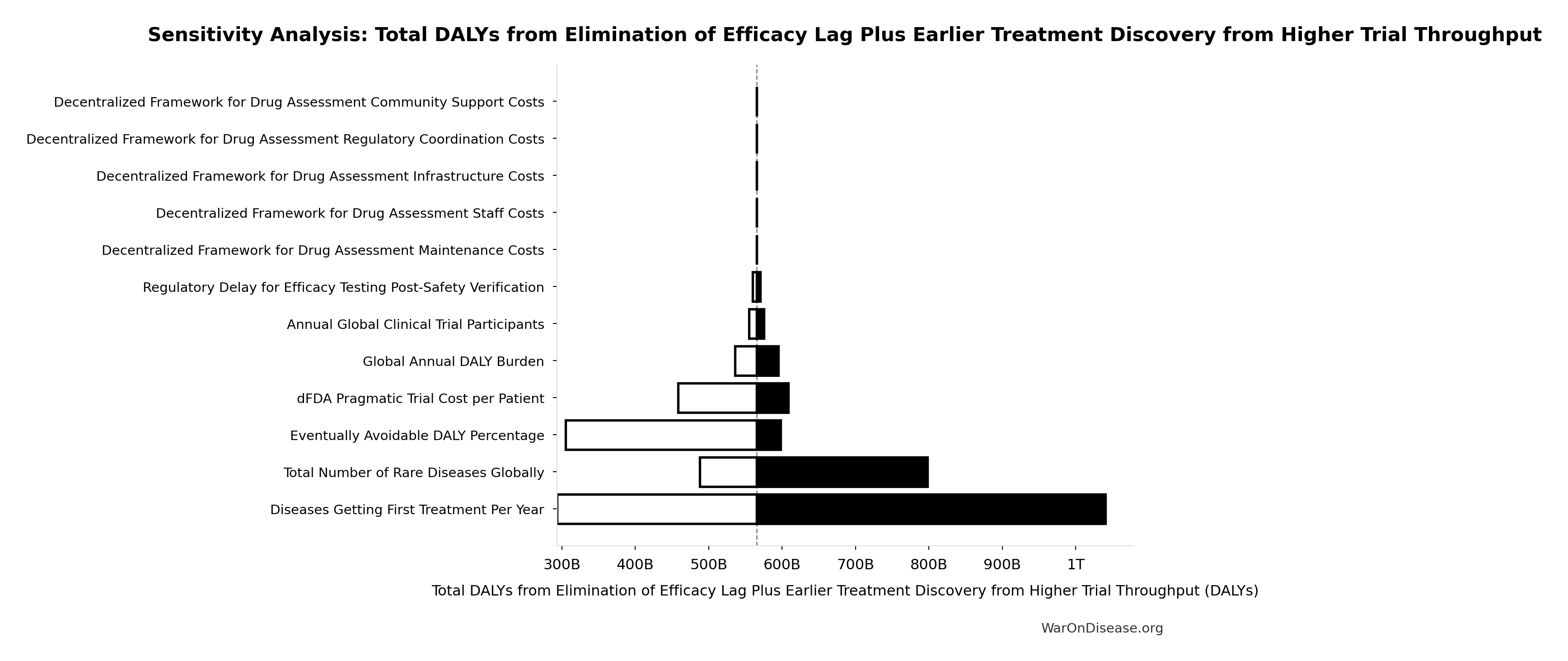
- Total DALYs from Elimination of Efficacy Lag Plus Earlier Treatment Discovery from Higher Trial Throughput 🔢: 565 billion DALYs
\[ DALYs_{pp} = DALYs_{max} \times 0.01 \]
✓ High confidence
Sensitivity Analysis
Sensitivity Indices for DALYs Averted per Percentage Point
Regression-based sensitivity showing which inputs explain the most variance in the output.
| Input Parameter | Sensitivity Coefficient | Interpretation |
|---|---|---|
| Total DALYs from Elimination of Efficacy Lag Plus Earlier Treatment Discovery from Higher Trial Throughput (DALYs) | 1.0000 | Strong driver |
Interpretation: Standardized coefficients show the change in output (in SD units) per 1 SD change in input. Values near ±1 indicate strong influence; values exceeding ±1 may occur with correlated inputs.
Monte Carlo Distribution
Simulation Results Summary: DALYs Averted per Percentage Point
| Statistic | Value |
|---|---|
| Baseline (deterministic) | 5.65 billion |
| Mean (expected value) | 6.1 billion |
| Median (50th percentile) | 6.14 billion |
| Standard Deviation | 1.48 billion |
| 90% Range (5th-95th percentile) | [3.61 billion, 8.77 billion] |
The histogram shows the distribution of DALYs Averted per Percentage Point across 10,000 Monte Carlo simulations. The CDF (right) shows the probability of the outcome exceeding any given value, which is useful for risk assessment.
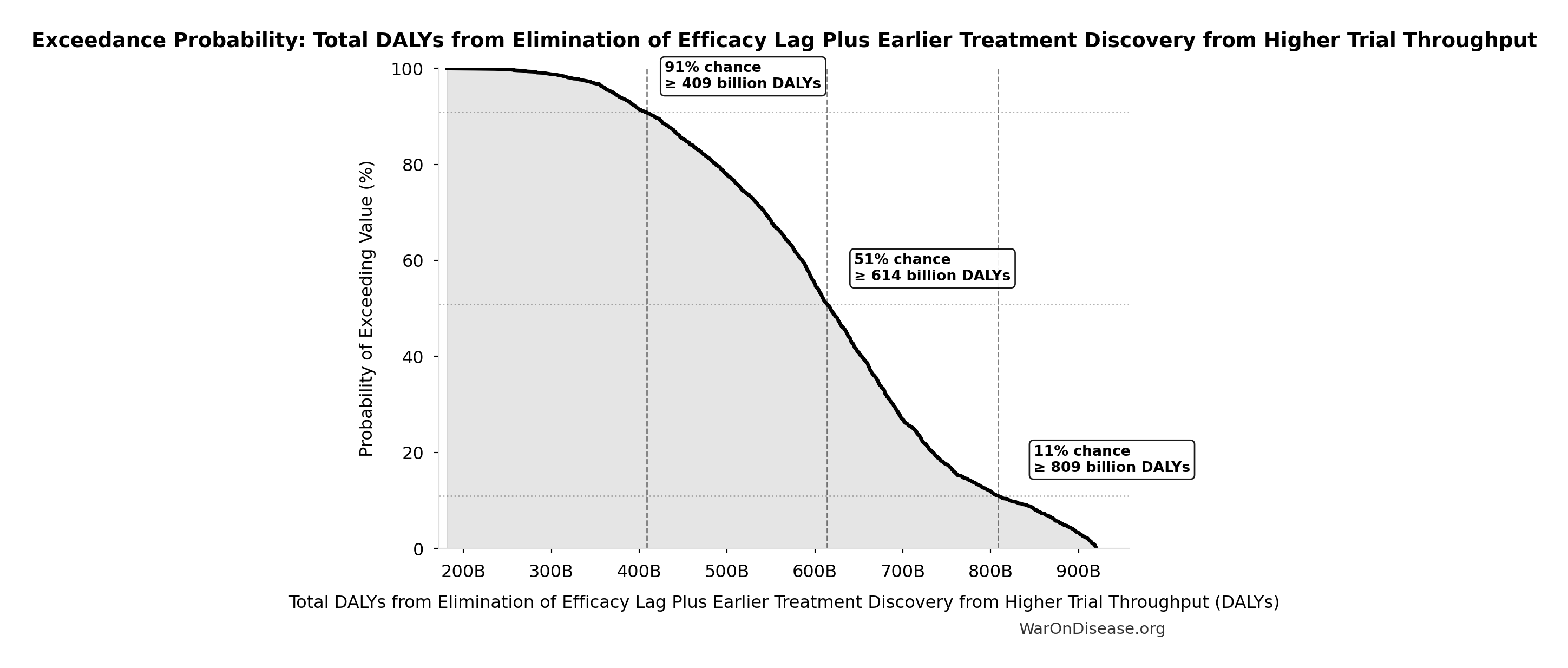
Exceedance Probability
This exceedance probability chart shows the likelihood that DALYs Averted per Percentage Point will exceed any given threshold. Higher curves indicate more favorable outcomes with greater certainty.
Contribution EV per Percentage Point (Treaty): $34.8K
Personal expected value per percentage point of implementation probability shift under Treaty Trajectory. One percent of the per-capita lifetime income gain.
Inputs:
\[ EV_{pp,treaty} = \Delta Y_{lifetime,treaty} \times 0.01 \]
✓ High confidence
Sensitivity Analysis
Sensitivity Indices for Contribution EV per Percentage Point (Treaty)
Regression-based sensitivity showing which inputs explain the most variance in the output.
| Input Parameter | Sensitivity Coefficient | Interpretation |
|---|---|---|
| Treaty Trajectory Lifetime Income Gain (Per Capita) (USD) | 1.0000 | Strong driver |
Interpretation: Standardized coefficients show the change in output (in SD units) per 1 SD change in input. Values near ±1 indicate strong influence; values exceeding ±1 may occur with correlated inputs.
Monte Carlo Distribution
Simulation Results Summary: Contribution EV per Percentage Point (Treaty)
| Statistic | Value |
|---|---|
| Baseline (deterministic) | $34.8K |
| Mean (expected value) | $40.6K |
| Median (50th percentile) | $33.5K |
| Standard Deviation | $26.6K |
| 90% Range (5th-95th percentile) | [$10.5K, $98.2K] |
The histogram shows the distribution of Contribution EV per Percentage Point (Treaty) across 10,000 Monte Carlo simulations. The CDF (right) shows the probability of the outcome exceeding any given value, which is useful for risk assessment.
Exceedance Probability
This exceedance probability chart shows the likelihood that Contribution EV per Percentage Point (Treaty) will exceed any given threshold. Higher curves indicate more favorable outcomes with greater certainty.
Contribution EV per Percentage Point (Treaty, Blended): $58.4K
Blended personal expected value per percentage point of implementation probability shift under Treaty Trajectory.
Inputs:
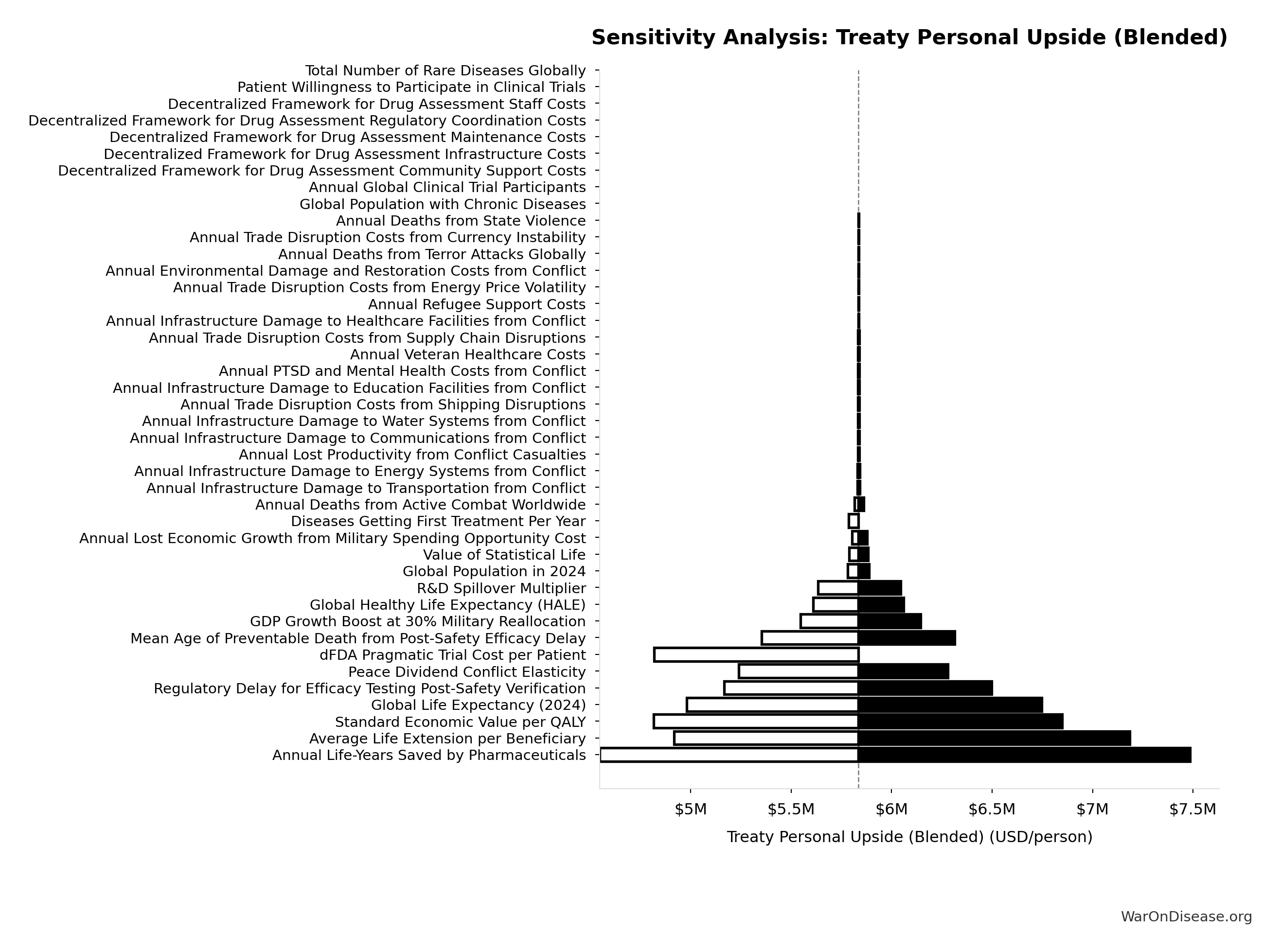
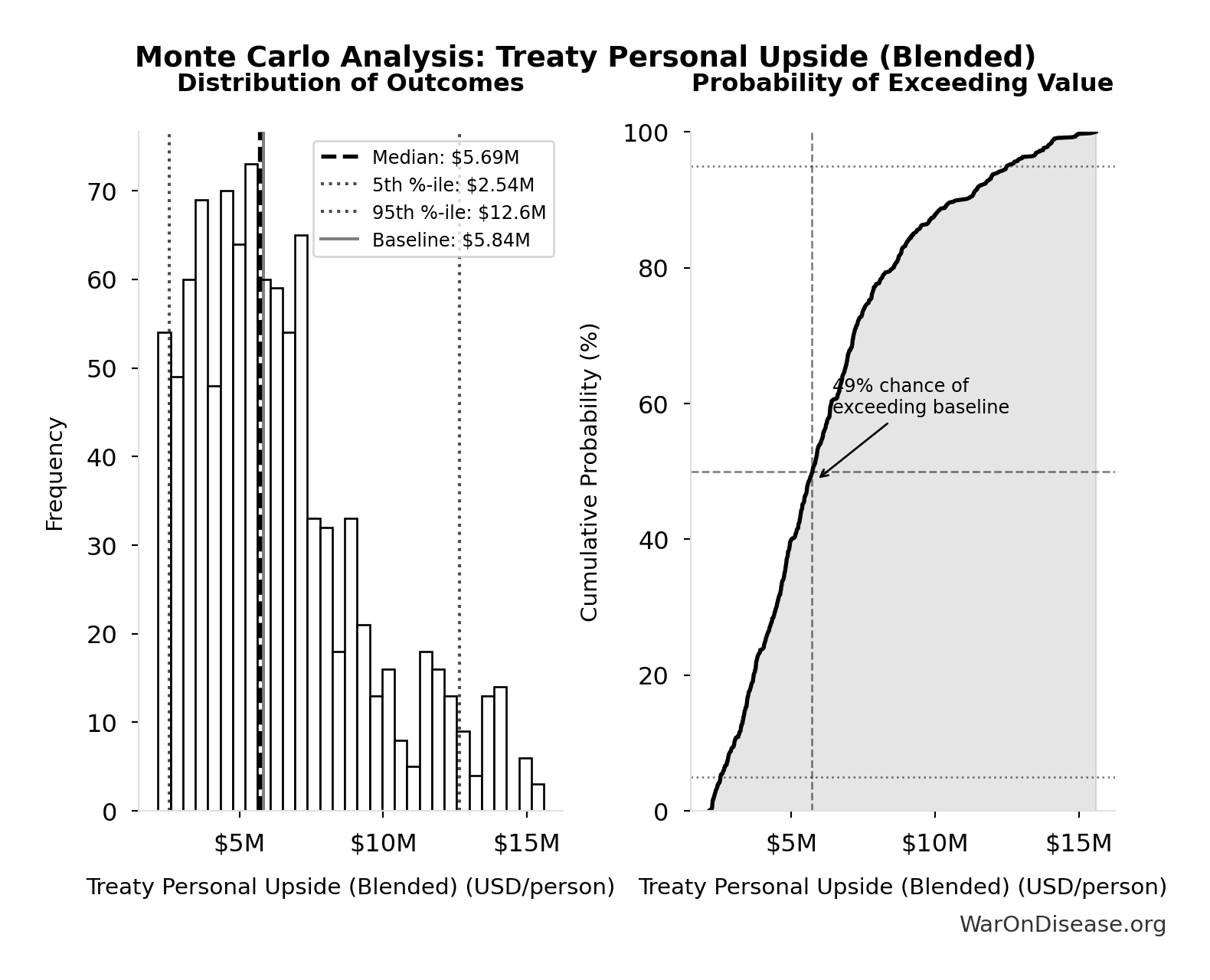
- Treaty Personal Upside (Blended) 🔢: $5.84M
\[ EV_{pp,treaty,blend} = Upside_{blend,treaty} \times 0.01 \]
✓ High confidence
Sensitivity Analysis
Sensitivity Indices for Contribution EV per Percentage Point (Treaty, Blended)
Regression-based sensitivity showing which inputs explain the most variance in the output.
| Input Parameter | Sensitivity Coefficient | Interpretation |
|---|---|---|
| Treaty Personal Upside (Blended) (USD/person) | 1.0000 | Strong driver |
Interpretation: Standardized coefficients show the change in output (in SD units) per 1 SD change in input. Values near ±1 indicate strong influence; values exceeding ±1 may occur with correlated inputs.
Monte Carlo Distribution
Simulation Results Summary: Contribution EV per Percentage Point (Treaty, Blended)
| Statistic | Value |
|---|---|
| Baseline (deterministic) | $58.4K |
| Mean (expected value) | $63.7K |
| Median (50th percentile) | $56.9K |
| Standard Deviation | $30.2K |
| 90% Range (5th-95th percentile) | [$25.4K, $126K] |
The histogram shows the distribution of Contribution EV per Percentage Point (Treaty, Blended) across 10,000 Monte Carlo simulations. The CDF (right) shows the probability of the outcome exceeding any given value, which is useful for risk assessment.
Exceedance Probability
This exceedance probability chart shows the likelihood that Contribution EV per Percentage Point (Treaty, Blended) will exceed any given threshold. Higher curves indicate more favorable outcomes with greater certainty.
Contribution EV per Percentage Point (Wishonia): $472K
Personal expected value per percentage point of implementation probability shift under Wishonia Trajectory. One percent of the per-capita lifetime income gain.
Inputs:
\[ EV_{pp,wish} = \Delta Y_{lifetime,wish} \times 0.01 \]
✓ High confidence
Sensitivity Analysis
Sensitivity Indices for Contribution EV per Percentage Point (Wishonia)
Regression-based sensitivity showing which inputs explain the most variance in the output.
| Input Parameter | Sensitivity Coefficient | Interpretation |
|---|---|---|
| Wishonia Trajectory Lifetime Income Gain (Per Capita) (USD) | 1.0000 | Strong driver |
Interpretation: Standardized coefficients show the change in output (in SD units) per 1 SD change in input. Values near ±1 indicate strong influence; values exceeding ±1 may occur with correlated inputs.
Monte Carlo Distribution
Simulation Results Summary: Contribution EV per Percentage Point (Wishonia)
| Statistic | Value |
|---|---|
| Baseline (deterministic) | $472K |
| Mean (expected value) | $820K |
| Median (50th percentile) | $468K |
| Standard Deviation | $965K |
| 90% Range (5th-95th percentile) | [$139K, $2.86M] |
The histogram shows the distribution of Contribution EV per Percentage Point (Wishonia) across 10,000 Monte Carlo simulations. The CDF (right) shows the probability of the outcome exceeding any given value, which is useful for risk assessment.
Exceedance Probability
This exceedance probability chart shows the likelihood that Contribution EV per Percentage Point (Wishonia) will exceed any given threshold. Higher curves indicate more favorable outcomes with greater certainty.
Contribution EV per Percentage Point (Wishonia, Blended): $496K
Blended personal expected value per percentage point of implementation probability shift under Wishonia Trajectory.
Inputs:
- Wishonia Personal Upside (Blended) 🔢: $49.6M
\[ EV_{pp,wish,blend} = Upside_{blend,wish} \times 0.01 \]
✓ High confidence
Sensitivity Analysis
Sensitivity Indices for Contribution EV per Percentage Point (Wishonia, Blended)
Regression-based sensitivity showing which inputs explain the most variance in the output.
| Input Parameter | Sensitivity Coefficient | Interpretation |
|---|---|---|
| Wishonia Personal Upside (Blended) (USD/person) | 1.0000 | Strong driver |
Interpretation: Standardized coefficients show the change in output (in SD units) per 1 SD change in input. Values near ±1 indicate strong influence; values exceeding ±1 may occur with correlated inputs.
Monte Carlo Distribution
Simulation Results Summary: Contribution EV per Percentage Point (Wishonia, Blended)
| Statistic | Value |
|---|---|
| Baseline (deterministic) | $496K |
| Mean (expected value) | $844K |
| Median (50th percentile) | $491K |
| Standard Deviation | $969K |
| 90% Range (5th-95th percentile) | [$154K, $2.9M] |
The histogram shows the distribution of Contribution EV per Percentage Point (Wishonia, Blended) across 10,000 Monte Carlo simulations. The CDF (right) shows the probability of the outcome exceeding any given value, which is useful for risk assessment.
Exceedance Probability
This exceedance probability chart shows the likelihood that Contribution EV per Percentage Point (Wishonia, Blended) will exceed any given threshold. Higher curves indicate more favorable outcomes with greater certainty.
Lives Saved per Percentage Point: 107 million lives
Lives saved per percentage point of implementation probability shift. One percent of total lives saved from eliminating trial capacity bottleneck and efficacy lag.
Inputs:
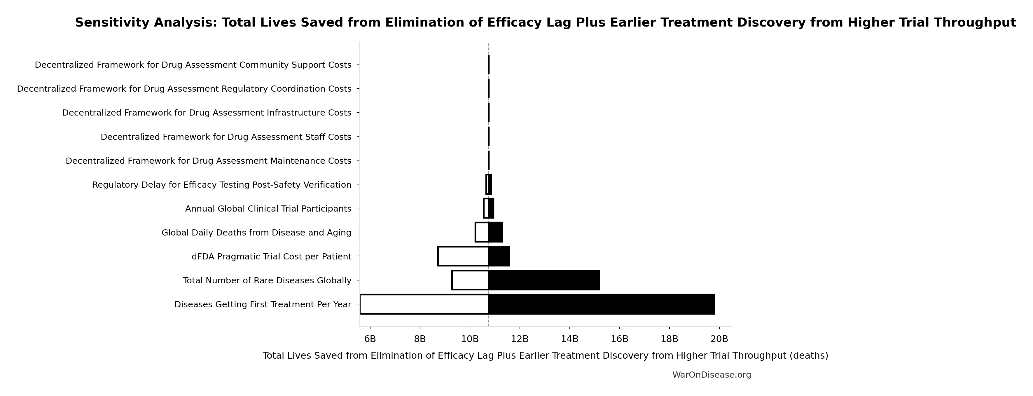
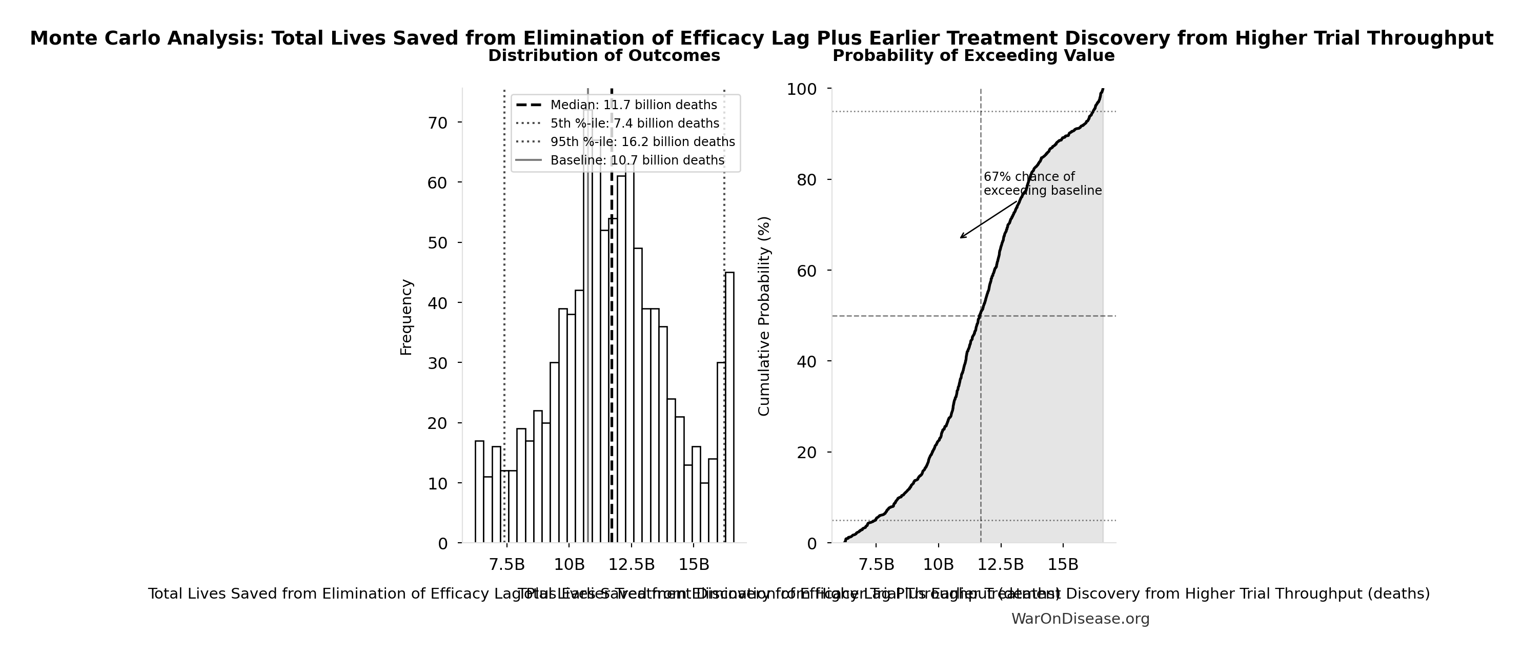
- Total Lives Saved from Elimination of Efficacy Lag Plus Earlier Treatment Discovery from Higher Trial Throughput 🔢: 10.7 billion deaths
\[ Lives_{pp} = Lives_{max} \times 0.01 \]
✓ High confidence
Sensitivity Analysis
Sensitivity Indices for Lives Saved per Percentage Point
Regression-based sensitivity showing which inputs explain the most variance in the output.
| Input Parameter | Sensitivity Coefficient | Interpretation |
|---|---|---|
| Total Lives Saved from Elimination of Efficacy Lag Plus Earlier Treatment Discovery from Higher Trial Throughput (deaths) | 1.0000 | Strong driver |
Interpretation: Standardized coefficients show the change in output (in SD units) per 1 SD change in input. Values near ±1 indicate strong influence; values exceeding ±1 may occur with correlated inputs.
Monte Carlo Distribution
Simulation Results Summary: Lives Saved per Percentage Point
| Statistic | Value |
|---|---|
| Baseline (deterministic) | 107 million |
| Mean (expected value) | 117 million |
| Median (50th percentile) | 117 million |
| Standard Deviation | 24.5 million |
| 90% Range (5th-95th percentile) | [74 million, 162 million] |
The histogram shows the distribution of Lives Saved per Percentage Point across 10,000 Monte Carlo simulations. The CDF (right) shows the probability of the outcome exceeding any given value, which is useful for risk assessment.
Exceedance Probability
This exceedance probability chart shows the likelihood that Lives Saved per Percentage Point will exceed any given threshold. Higher curves indicate more favorable outcomes with greater certainty.
Suffering Hours Prevented per Percentage Point: 19.3 trillion hours
Suffering hours prevented per percentage point of implementation probability shift. One percent of total suffering hours from eliminating trial capacity bottleneck and efficacy lag.
Inputs:
- Suffering Hours Eliminated from Elimination of Efficacy Lag Plus Earlier Treatment Discovery from Higher Trial Throughput 🔢: 1.93 quadrillion hours
\[ Hours_{pp} = Hours_{suffer,max} \times 0.01 \]
✓ High confidence
Sensitivity Analysis
Sensitivity Indices for Suffering Hours Prevented per Percentage Point
Regression-based sensitivity showing which inputs explain the most variance in the output.
| Input Parameter | Sensitivity Coefficient | Interpretation |
|---|---|---|
| Suffering Hours Eliminated from Elimination of Efficacy Lag Plus Earlier Treatment Discovery from Higher Trial Throughput (hours) | 1.0000 | Strong driver |
Interpretation: Standardized coefficients show the change in output (in SD units) per 1 SD change in input. Values near ±1 indicate strong influence; values exceeding ±1 may occur with correlated inputs.
Monte Carlo Distribution
Simulation Results Summary: Suffering Hours Prevented per Percentage Point
| Statistic | Value |
|---|---|
| Baseline (deterministic) | 19.3 trillion |
| Mean (expected value) | 20.5 trillion |
| Median (50th percentile) | 21.1 trillion |
| Standard Deviation | 3.74 trillion |
| 90% Range (5th-95th percentile) | [13.6 trillion, 26.2 trillion] |
The histogram shows the distribution of Suffering Hours Prevented per Percentage Point across 10,000 Monte Carlo simulations. The CDF (right) shows the probability of the outcome exceeding any given value, which is useful for risk assessment.
Exceedance Probability
This exceedance probability chart shows the likelihood that Suffering Hours Prevented per Percentage Point will exceed any given threshold. Higher curves indicate more favorable outcomes with greater certainty.
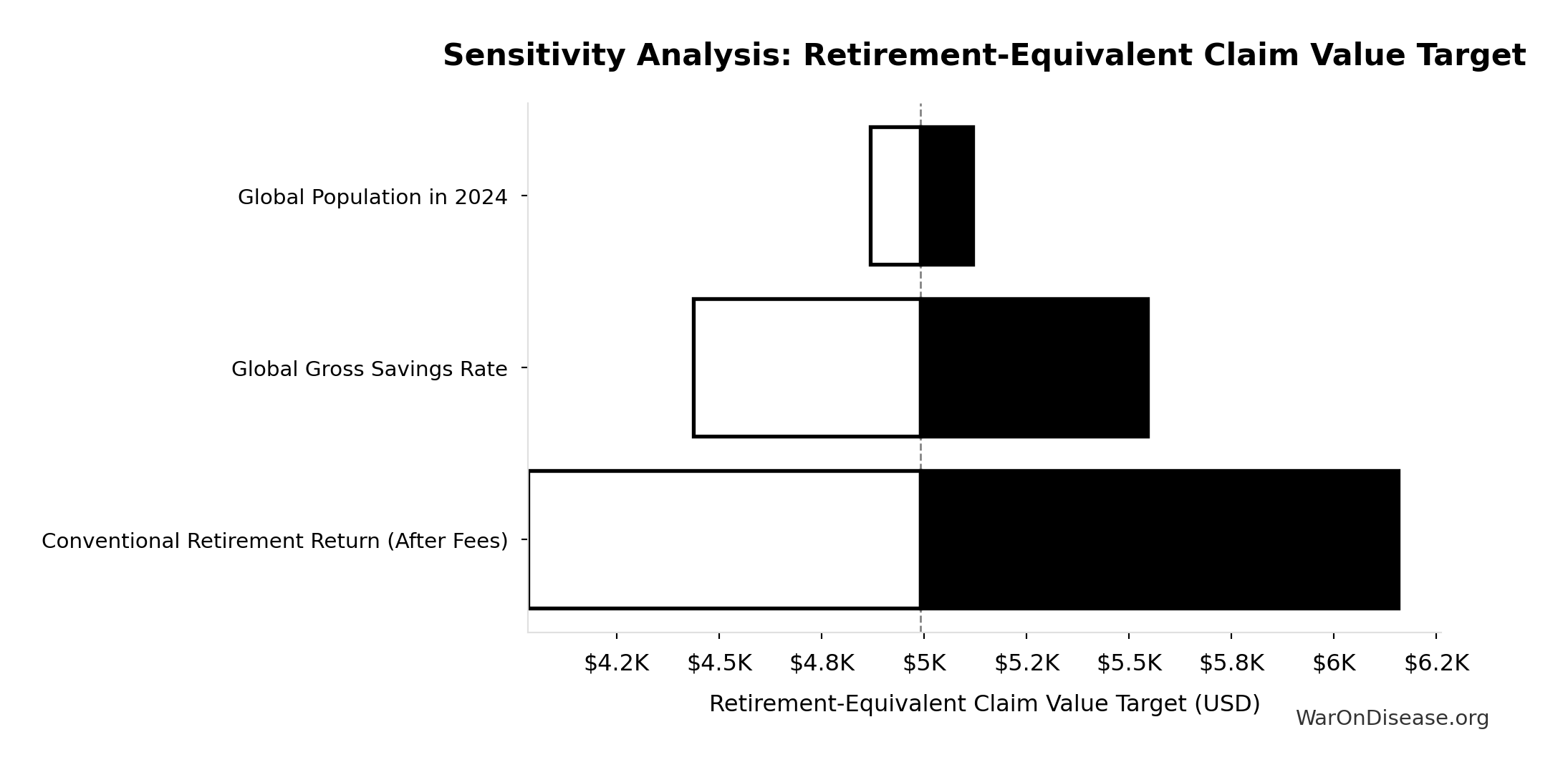
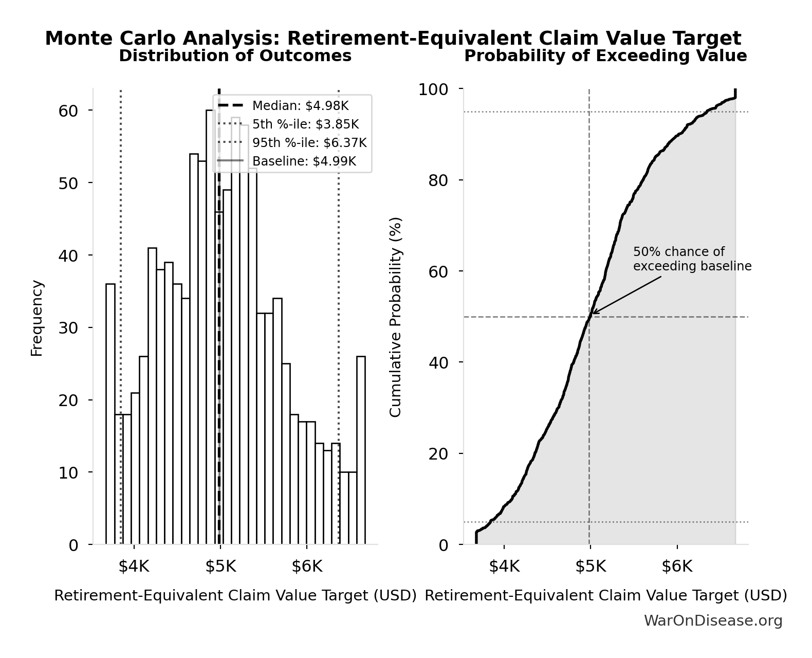
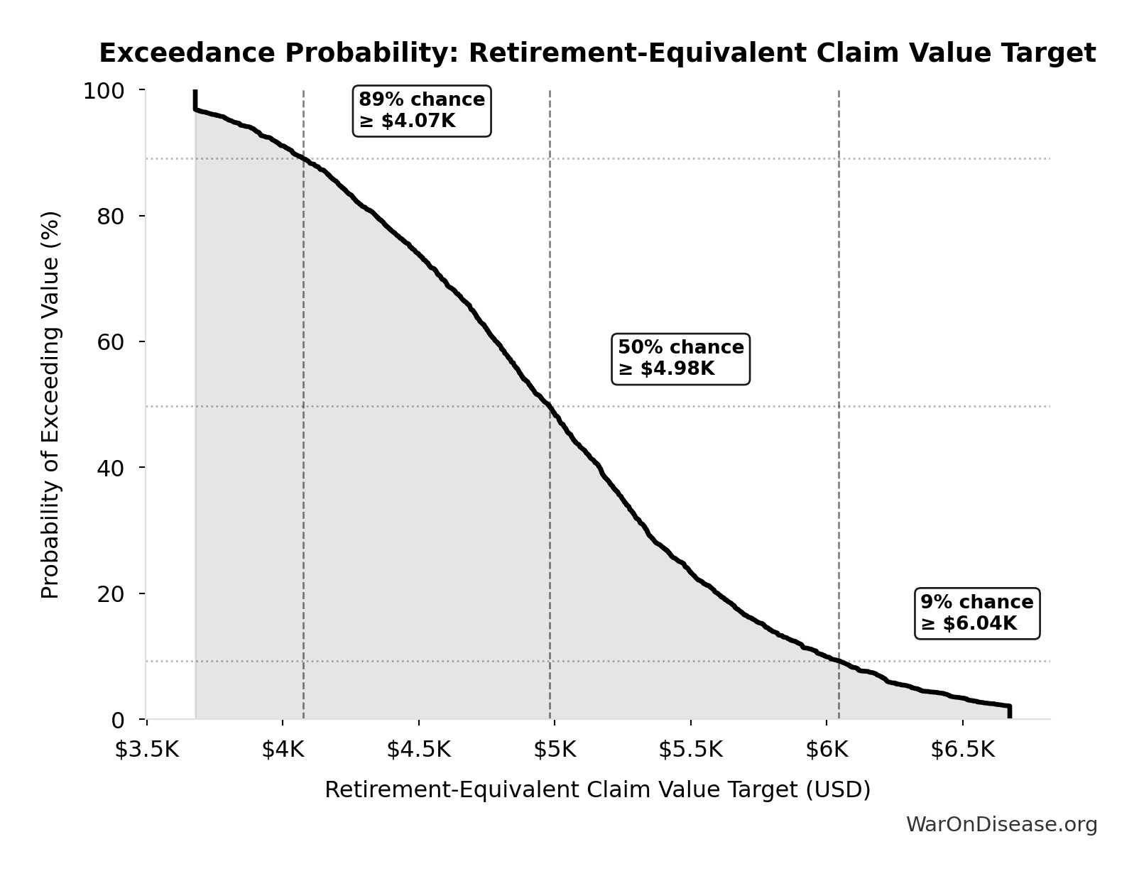
Conventional Retirement Horizon Multiple: 2.57x
Compound multiple for conventional retirement investing over the PRIZE pool resolution horizon (tied to the destructive economy 50% threshold year).
Inputs:
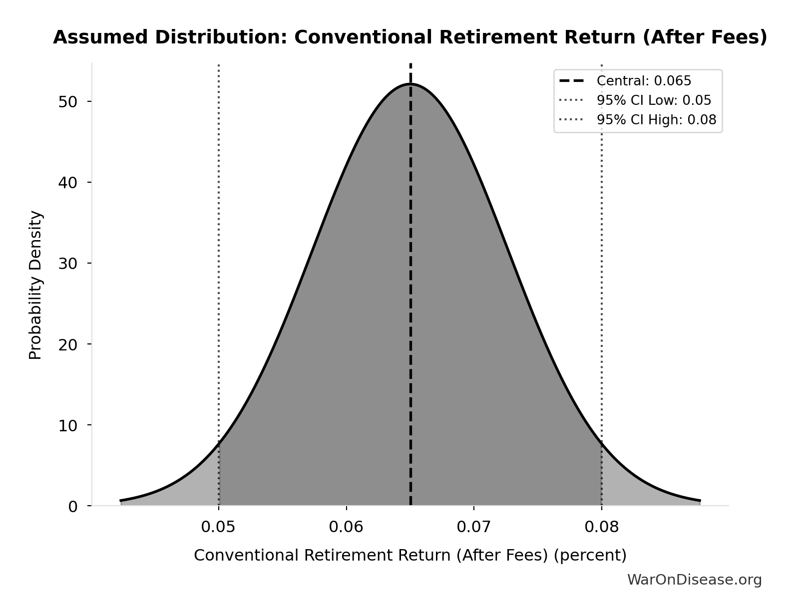
- Conventional Retirement Return (After Fees) 📊: 6.5% (95% CI: 5% - 8%)
- Year Destructive Economy Reaches 50% of GDP 🔢: 2040
- Destructive Economy Base Year: 2025
\[ M_{retire} = (1 + r_{retire})^{Y_{50\%} - Y_0} \]
✓ High confidence
Sensitivity Analysis
Sensitivity Indices for Conventional Retirement Horizon Multiple
Regression-based sensitivity showing which inputs explain the most variance in the output.
| Input Parameter | Sensitivity Coefficient | Interpretation |
|---|---|---|
| Conventional Retirement Return (After Fees) (percent) | 0.9983 | Strong driver |
Interpretation: Standardized coefficients show the change in output (in SD units) per 1 SD change in input. Values near ±1 indicate strong influence; values exceeding ±1 may occur with correlated inputs.
Monte Carlo Distribution
Simulation Results Summary: Conventional Retirement Horizon Multiple
| Statistic | Value |
|---|---|
| Baseline (deterministic) | 2.57x |
| Mean (expected value) | 2.58x |
| Median (50th percentile) | 2.57x |
| Standard Deviation | 0.267x |
| 90% Range (5th-95th percentile) | [2.14x, 3.07x] |
The histogram shows the distribution of Conventional Retirement Horizon Multiple across 10,000 Monte Carlo simulations. The CDF (right) shows the probability of the outcome exceeding any given value, which is useful for risk assessment.
Exceedance Probability
This exceedance probability chart shows the likelihood that Conventional Retirement Horizon Multiple will exceed any given threshold. Higher curves indicate more favorable outcomes with greater certainty.
Combination Therapy Exploration Time (Current): 13.7 million years
Years to test all pairwise drug combinations at current trial capacity. Combination therapy is standard in oncology, HIV, cardiology.
Inputs:
- Combination Therapy Space 🔢: 45.1 billion combinations
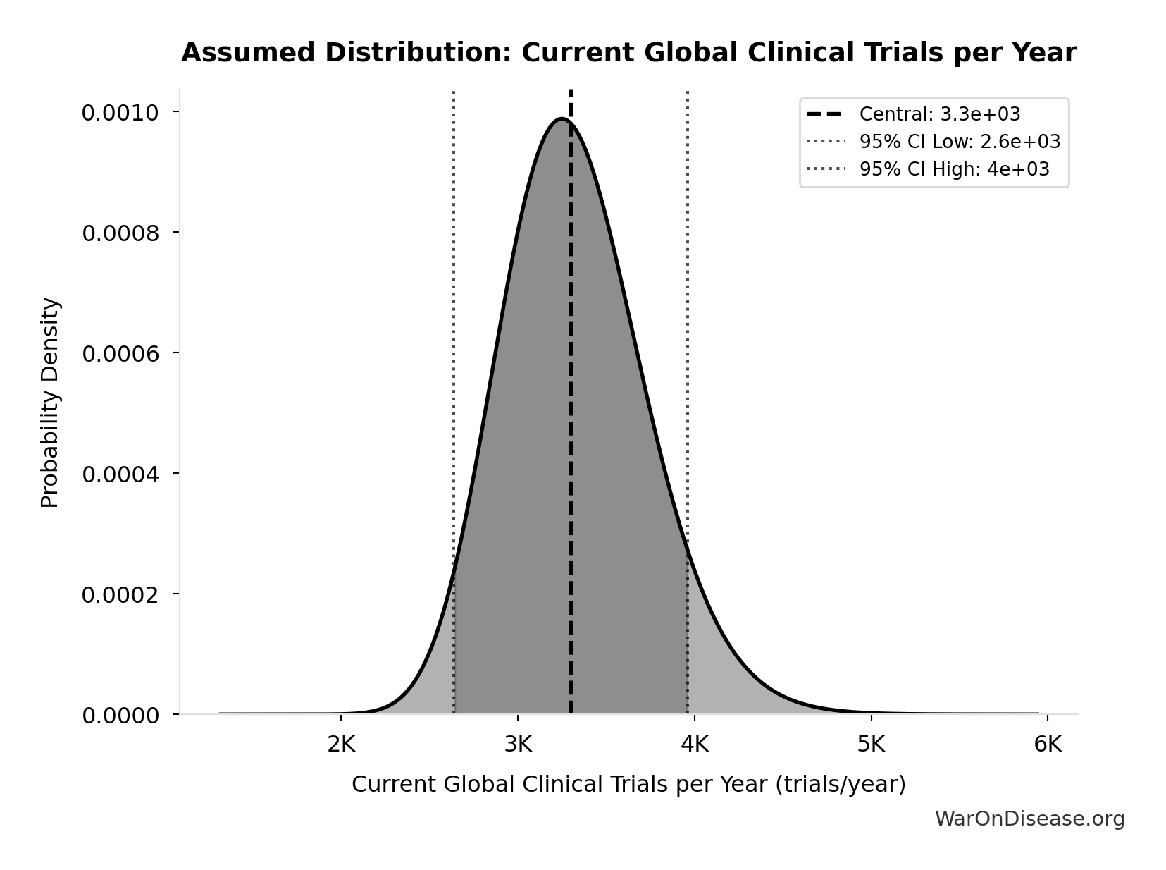
- Current Global Clinical Trials per Year 📊: 3.3 thousand trials/year (95% CI: 2.64 thousand trials/year - 3.96 thousand trials/year)
\[ \begin{gathered} T_{explore,combo} \\ = \frac{Space_{combo}}{Trials_{ann,curr}} \\ = \frac{45.1B}{3{,}300} \\ = 13.7M \end{gathered} \] where: \[ \begin{gathered} Space_{combo} \\ = N_{combo} \times N_{diseases,trial} \\ = 45.1M \times 1{,}000 \\ = 45.1B \end{gathered} \] ✓ High confidence
Sensitivity Analysis
Sensitivity Indices for Combination Therapy Exploration Time (Current)
Regression-based sensitivity showing which inputs explain the most variance in the output.
| Input Parameter | Sensitivity Coefficient | Interpretation |
|---|---|---|
| Current Global Clinical Trials per Year (trials/year) | -0.9931 | Strong driver |
Interpretation: Standardized coefficients show the change in output (in SD units) per 1 SD change in input. Values near ±1 indicate strong influence; values exceeding ±1 may occur with correlated inputs.
Monte Carlo Distribution
Simulation Results Summary: Combination Therapy Exploration Time (Current)
| Statistic | Value |
|---|---|
| Baseline (deterministic) | 13.7 million |
| Mean (expected value) | 13.8 million |
| Median (50th percentile) | 13.8 million |
| Standard Deviation | 1.36 million |
| 90% Range (5th-95th percentile) | [11.6 million, 16.3 million] |
The histogram shows the distribution of Combination Therapy Exploration Time (Current) across 10,000 Monte Carlo simulations. The CDF (right) shows the probability of the outcome exceeding any given value, which is useful for risk assessment.
Exceedance Probability
This exceedance probability chart shows the likelihood that Combination Therapy Exploration Time (Current) will exceed any given threshold. Higher curves indicate more favorable outcomes with greater certainty.
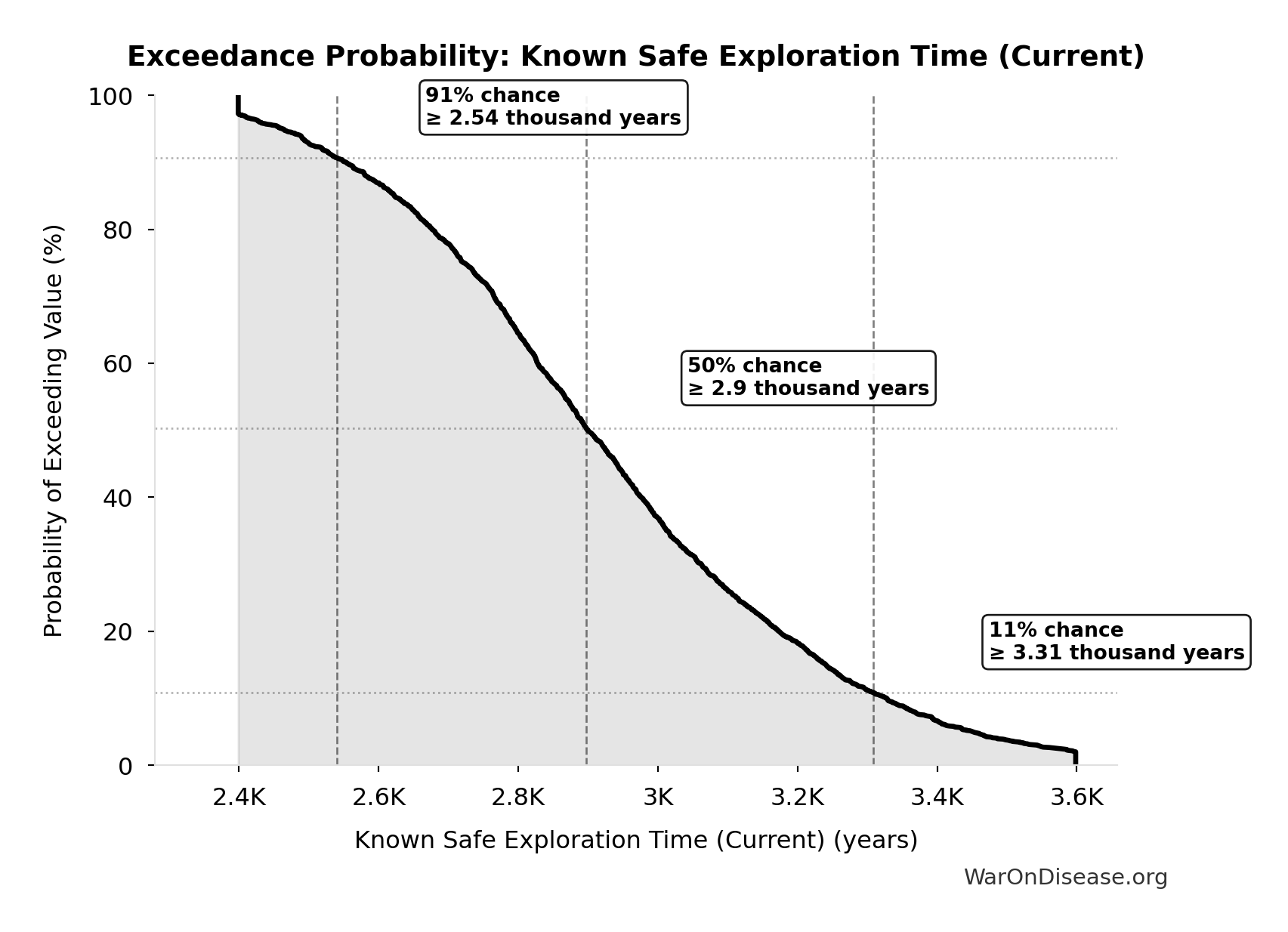
Known Safe Exploration Time (Current): 2.88 thousand years
Years to test all known safe drug-disease combinations at current global trial capacity
Inputs:
- Possible Drug-Disease Combinations 🔢: 9.5 million combinations
- Current Global Clinical Trials per Year 📊: 3.3 thousand trials/year (95% CI: 2.64 thousand trials/year - 3.96 thousand trials/year)
\[ \begin{gathered} T_{explore,safe} \\ = \frac{N_{combos}}{Trials_{ann,curr}} \\ = \frac{9.5M}{3{,}300} \\ = 2{,}880 \end{gathered} \] where: \[ \begin{gathered} N_{combos} \\ = N_{safe} \times N_{diseases,trial} \\ = 9{,}500 \times 1{,}000 \\ = 9.5M \end{gathered} \] ✓ High confidence
Sensitivity Analysis
Sensitivity Indices for Known Safe Exploration Time (Current)
Regression-based sensitivity showing which inputs explain the most variance in the output.
| Input Parameter | Sensitivity Coefficient | Interpretation |
|---|---|---|
| Current Global Clinical Trials per Year (trials/year) | -0.9931 | Strong driver |
Interpretation: Standardized coefficients show the change in output (in SD units) per 1 SD change in input. Values near ±1 indicate strong influence; values exceeding ±1 may occur with correlated inputs.
Monte Carlo Distribution
Simulation Results Summary: Known Safe Exploration Time (Current)
| Statistic | Value |
|---|---|
| Baseline (deterministic) | 2.88 thousand |
| Mean (expected value) | 2.91 thousand |
| Median (50th percentile) | 2.9 thousand |
| Standard Deviation | 286 |
| 90% Range (5th-95th percentile) | [2.45 thousand, 3.43 thousand] |
The histogram shows the distribution of Known Safe Exploration Time (Current) across 10,000 Monte Carlo simulations. The CDF (right) shows the probability of the outcome exceeding any given value, which is useful for risk assessment.
Exceedance Probability
This exceedance probability chart shows the likelihood that Known Safe Exploration Time (Current) will exceed any given threshold. Higher curves indicate more favorable outcomes with greater certainty.
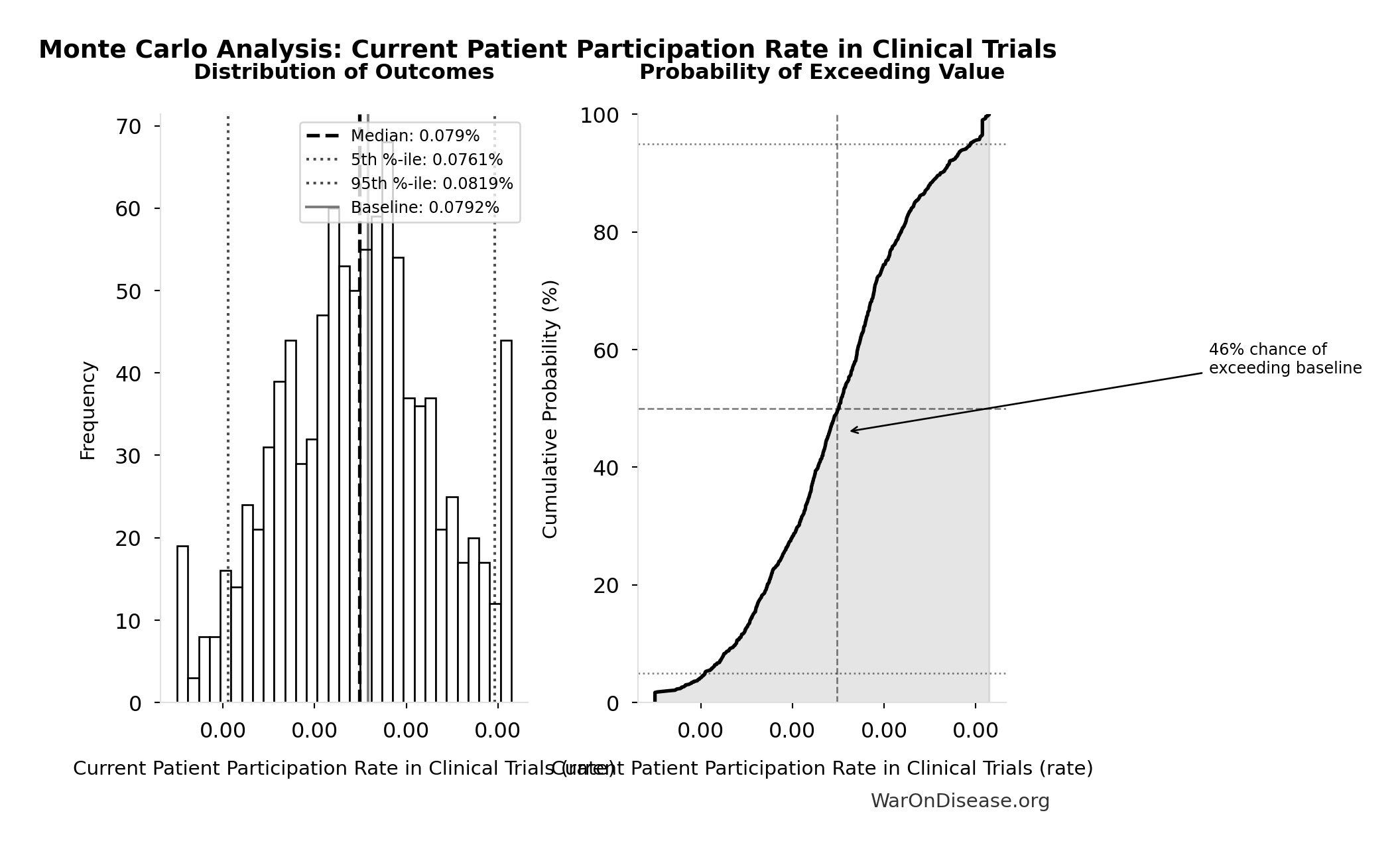
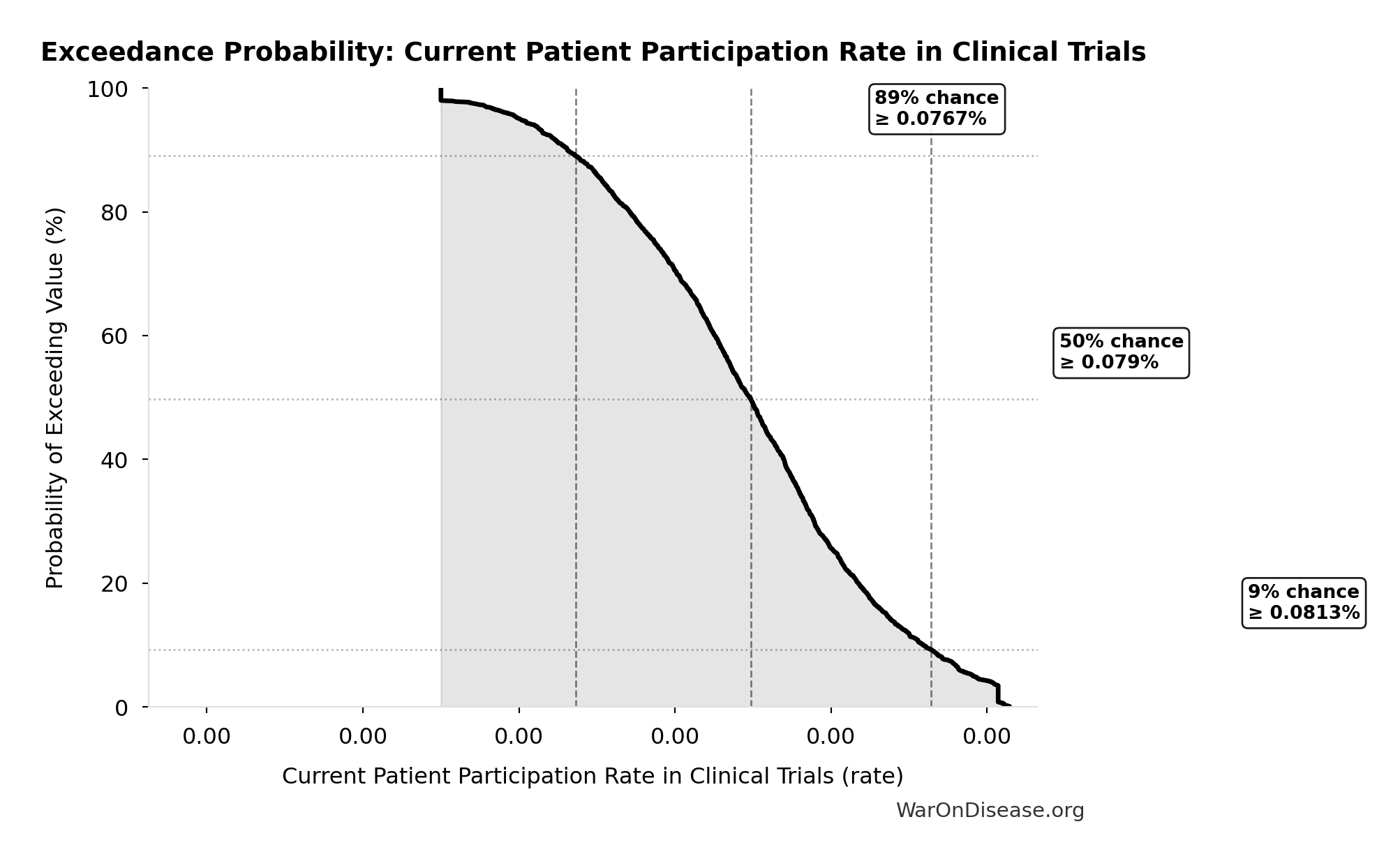
Current Patient Participation Rate in Clinical Trials: 0.0792%
Current patient participation rate in clinical trials (0.08% = 1.9M participants / 2.4B disease patients)
Inputs:
- Annual Global Clinical Trial Participants 📊: 1.9 million patients/year (95% CI: 1.5 million patients/year - 2.3 million patients/year)
- Global Population with Chronic Diseases 📊: 2.4 billion people (95% CI: 2 billion people - 2.8 billion people)
\[ \begin{gathered} Rate_{part} \\ = \frac{Slots_{curr}}{N_{patients}} \\ = \frac{1.9M}{2.4B} \\ = 0.0792\% \end{gathered} \]
Methodology:13
✓ High confidence
Sensitivity Analysis
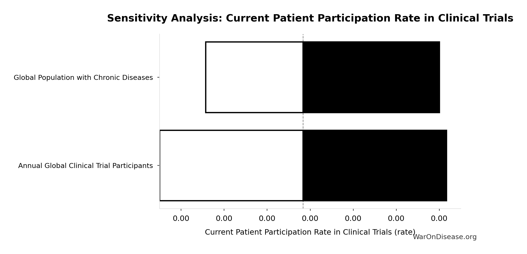
Sensitivity Indices for Current Patient Participation Rate in Clinical Trials
Regression-based sensitivity showing which inputs explain the most variance in the output.
| Input Parameter | Sensitivity Coefficient | Interpretation |
|---|---|---|
| Global Population with Chronic Diseases (people) | 4.1698 | Strong driver |
| Annual Global Clinical Trial Participants (patients/year) | -3.1720 | Strong driver |
Interpretation: Standardized coefficients show the change in output (in SD units) per 1 SD change in input. Values near ±1 indicate strong influence; values exceeding ±1 may occur with correlated inputs.
Monte Carlo Distribution
Simulation Results Summary: Current Patient Participation Rate in Clinical Trials
| Statistic | Value |
|---|---|
| Baseline (deterministic) | 0.0792% |
| Mean (expected value) | 0.079% |
| Median (50th percentile) | 0.079% |
| Standard Deviation | 0.00169% |
| 90% Range (5th-95th percentile) | [0.0761%, 0.0819%] |
The histogram shows the distribution of Current Patient Participation Rate in Clinical Trials across 10,000 Monte Carlo simulations. The CDF (right) shows the probability of the outcome exceeding any given value, which is useful for risk assessment.
Exceedance Probability
This exceedance probability chart shows the likelihood that Current Patient Participation Rate in Clinical Trials will exceed any given threshold. Higher curves indicate more favorable outcomes with greater certainty.
Current Trajectory Average Income at Year 15: $18.7K
Average income (GDP per capita) at year 15 under current trajectory.
Inputs:
- Current Trajectory GDP at Year 15 🔢: $167T
- Global Population 2040 (Projected) 📊: 8.9 billion of people
\[ \bar{y}_{base,15} = \frac{GDP_{base,15}}{Pop_{2040}} \]
✓ High confidence
Monte Carlo Distribution
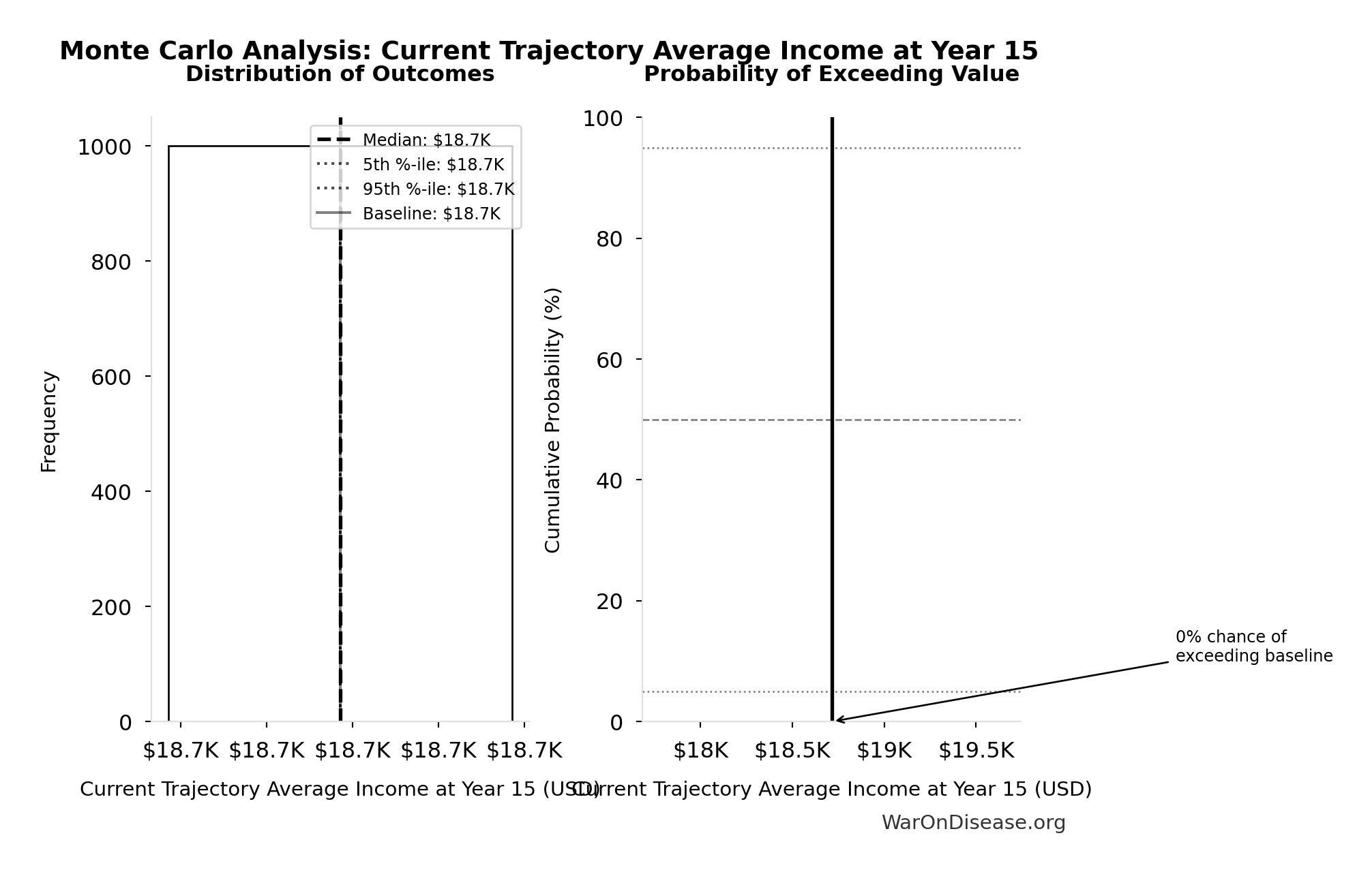
Simulation Results Summary: Current Trajectory Average Income at Year 15
| Statistic | Value |
|---|---|
| Baseline (deterministic) | $18.7K |
| Mean (expected value) | $18.7K |
| Median (50th percentile) | $18.7K |
| Standard Deviation | $3.64e-12 |
| 90% Range (5th-95th percentile) | [$18.7K, $18.7K] |
The histogram shows the distribution of Current Trajectory Average Income at Year 15 across 10,000 Monte Carlo simulations. The CDF (right) shows the probability of the outcome exceeding any given value, which is useful for risk assessment.
Exceedance Probability
This exceedance probability chart shows the likelihood that Current Trajectory Average Income at Year 15 will exceed any given threshold. Higher curves indicate more favorable outcomes with greater certainty.
Current Trajectory Average Income at Year 20: $20.5K
Average income (GDP per capita) at year 20 under current trajectory trajectory.
Inputs:
- Current Trajectory GDP at Year 20 🔢: $188T
- Global Population 2045 (Projected) 📊: 9.2 billion of people
\[ \begin{gathered} \bar{y}_{base,20} \\ = \frac{GDP_{base,20}}{Pop_{2045}} \\ = \frac{\$188T}{9.2B} \\ = \$20.5K \end{gathered} \] where: \[ GDP_{base,20} = GDP_0(1+g_{base})^{20} \] ✓ High confidence
Monte Carlo Distribution
Simulation Results Summary: Current Trajectory Average Income at Year 20
| Statistic | Value |
|---|---|
| Baseline (deterministic) | $20.5K |
| Mean (expected value) | $20.5K |
| Median (50th percentile) | $20.5K |
| Standard Deviation | $3.64e-12 |
| 90% Range (5th-95th percentile) | [$20.5K, $20.5K] |
The histogram shows the distribution of Current Trajectory Average Income at Year 20 across 10,000 Monte Carlo simulations. The CDF (right) shows the probability of the outcome exceeding any given value, which is useful for risk assessment.
Exceedance Probability
This exceedance probability chart shows the likelihood that Current Trajectory Average Income at Year 20 will exceed any given threshold. Higher curves indicate more favorable outcomes with greater certainty.
Current Trajectory Cumulative Lifetime Income (Per Capita): $1.1M
Cumulative per-capita income over an average remaining lifespan under current trajectory baseline trajectory. Uses the implied per-capita baseline CAGR from 2025 to 2045.
Inputs:
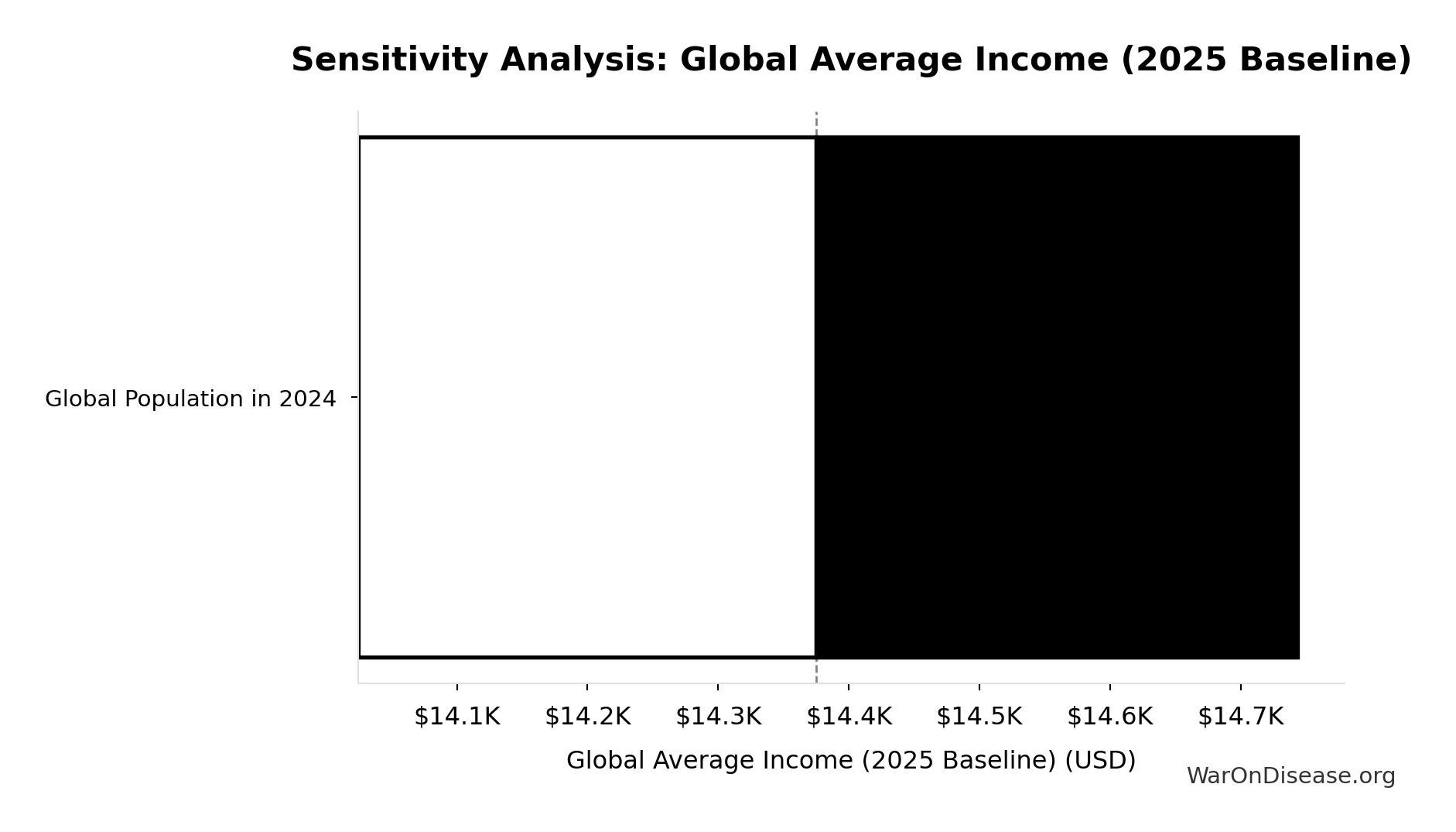
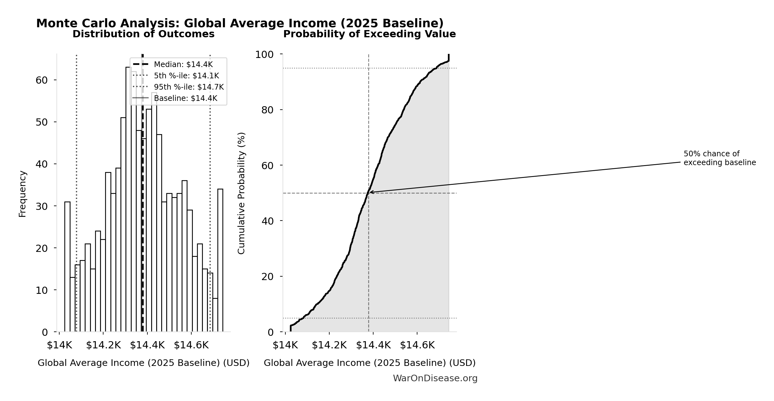
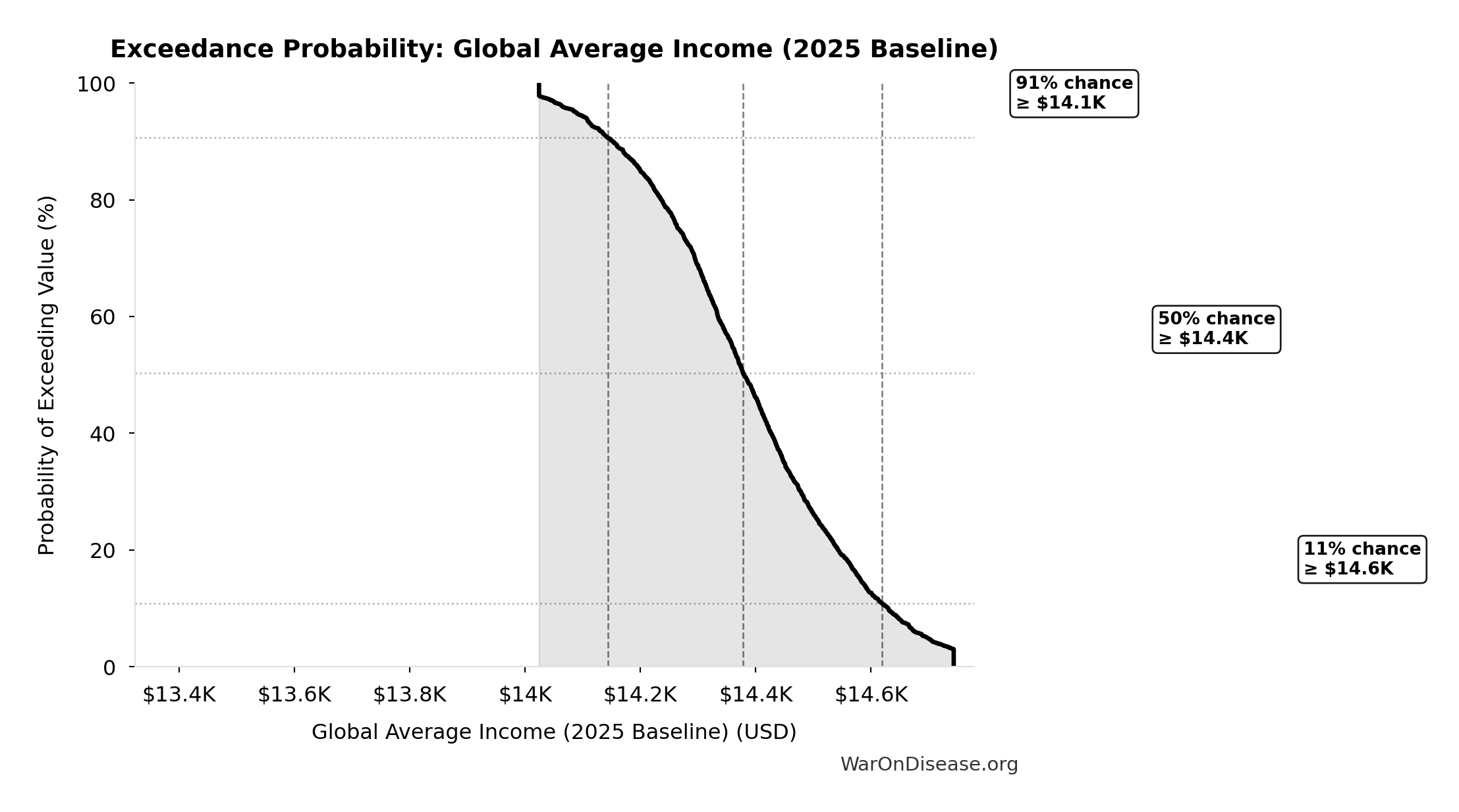
- Global Average Income (2025 Baseline) 🔢: $14.4K
- Current Trajectory Average Income at Year 20 🔢: $20.5K
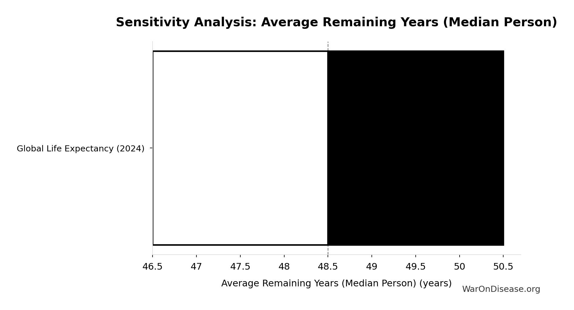
- Average Remaining Years (Median Person) 🔢: 48.5 years
\[ \begin{gathered} Y_{cum,earth} \\ = \bar{y}_0 \cdot \frac{(1+g_{pc,base})((1+g_{pc,base})^{T_{remaining}}-1)}{g_{pc,base}} \end{gathered} \]
✓ High confidence
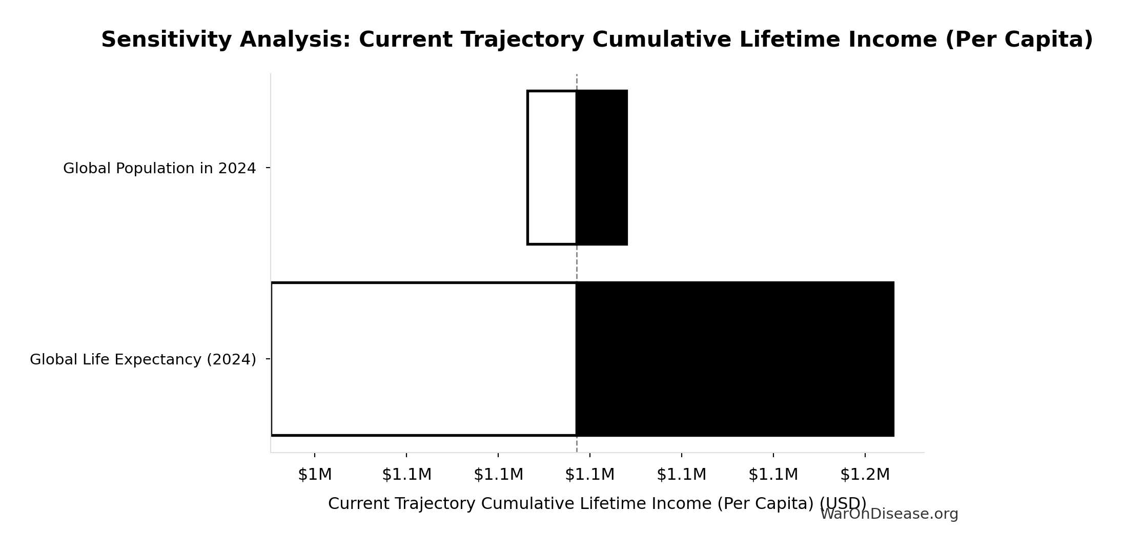
Sensitivity Analysis
Sensitivity Indices for Current Trajectory Cumulative Lifetime Income (Per Capita)
Regression-based sensitivity showing which inputs explain the most variance in the output.
| Input Parameter | Sensitivity Coefficient | Interpretation |
|---|---|---|
| Average Remaining Years (Median Person) (years) | 0.9477 | Strong driver |
| Global Average Income (2025 Baseline) (USD) | -0.0428 | Minimal effect |
Interpretation: Standardized coefficients show the change in output (in SD units) per 1 SD change in input. Values near ±1 indicate strong influence; values exceeding ±1 may occur with correlated inputs.
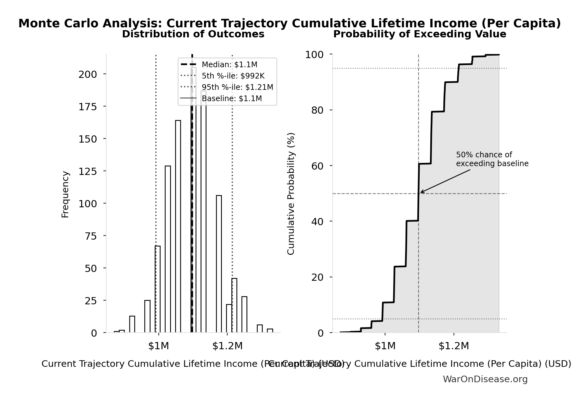
Monte Carlo Distribution
Simulation Results Summary: Current Trajectory Cumulative Lifetime Income (Per Capita)
| Statistic | Value |
|---|---|
| Baseline (deterministic) | $1.1M |
| Mean (expected value) | $1.1M |
| Median (50th percentile) | $1.1M |
| Standard Deviation | $74.3K |
| 90% Range (5th-95th percentile) | [$992K, $1.21M] |
The histogram shows the distribution of Current Trajectory Cumulative Lifetime Income (Per Capita) across 10,000 Monte Carlo simulations. The CDF (right) shows the probability of the outcome exceeding any given value, which is useful for risk assessment.
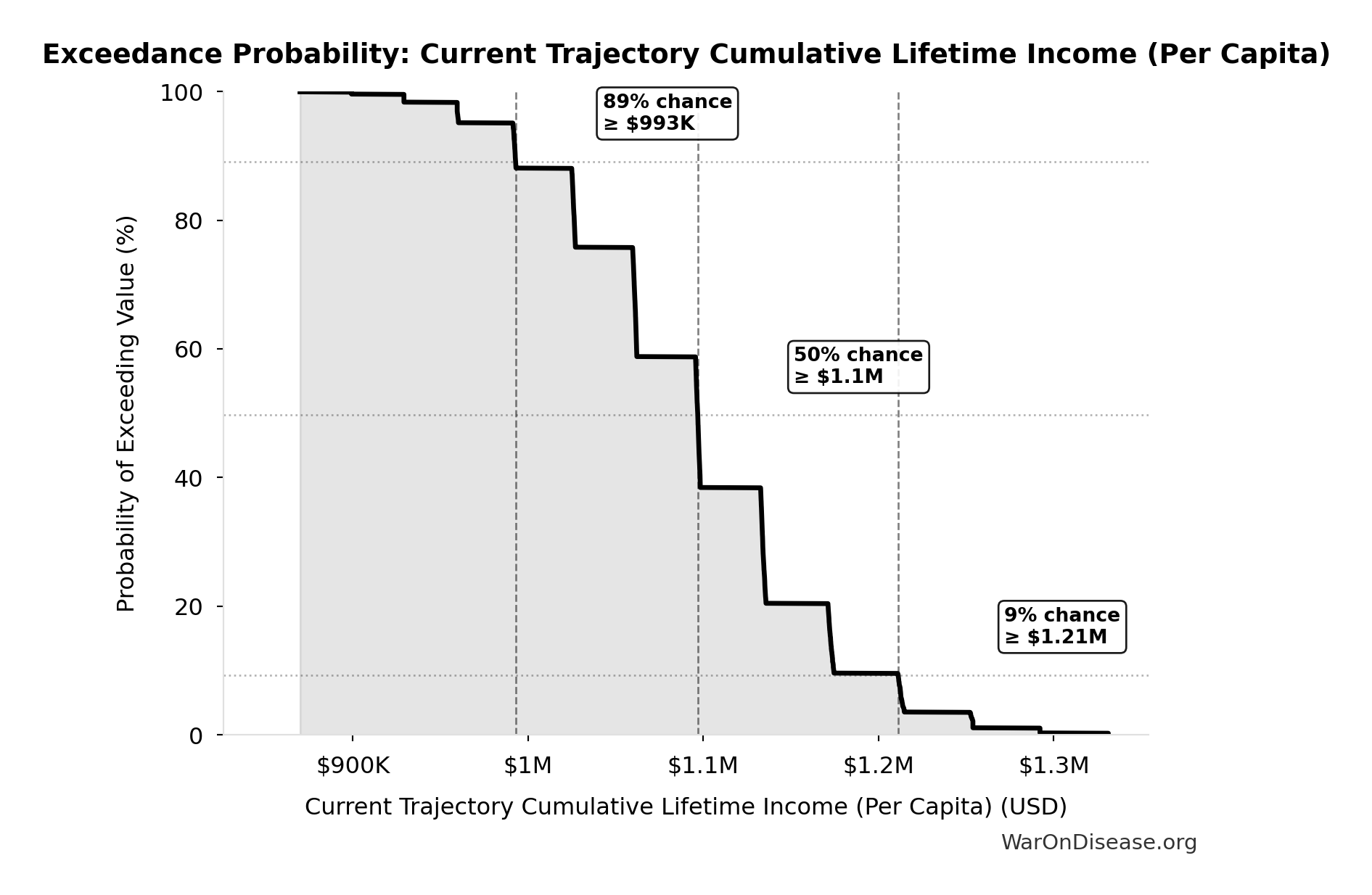
Exceedance Probability
This exceedance probability chart shows the likelihood that Current Trajectory Cumulative Lifetime Income (Per Capita) will exceed any given threshold. Higher curves indicate more favorable outcomes with greater certainty.
Current Trajectory GDP at Year 15: $167T
Global GDP at year 15 under status-quo current trajectory growth.
Inputs:
- Global GDP (2025) 📊: $115T
- Baseline Global GDP Growth Rate: 2.5%
\[ GDP_{base,15} = GDP_0(1+g_{base})^{15} \]
✓ High confidence
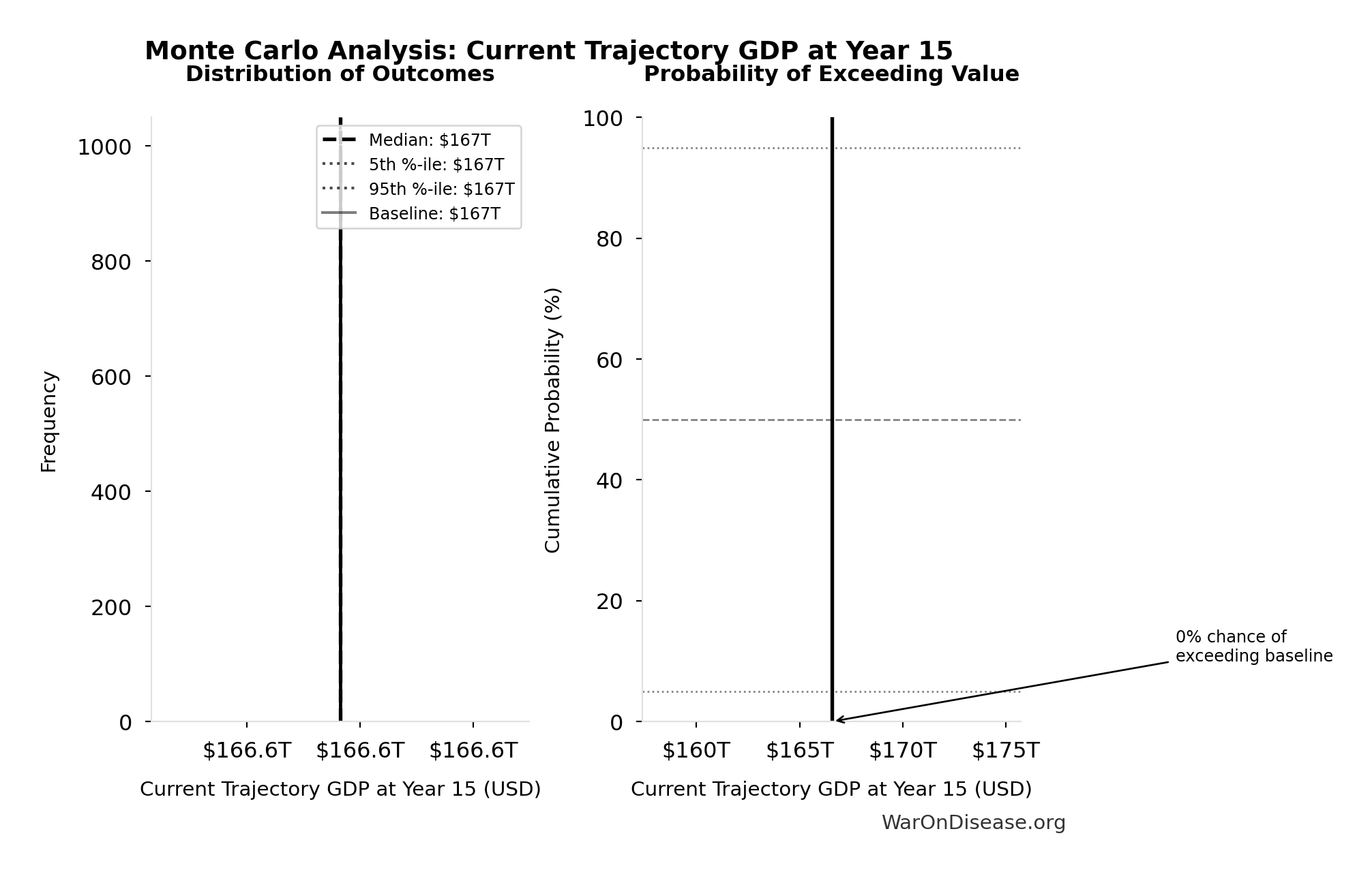
Monte Carlo Distribution
Simulation Results Summary: Current Trajectory GDP at Year 15
| Statistic | Value |
|---|---|
| Baseline (deterministic) | $167T |
| Mean (expected value) | $167T |
| Median (50th percentile) | $167T |
| Standard Deviation | $0.031 |
| 90% Range (5th-95th percentile) | [$167T, $167T] |
The histogram shows the distribution of Current Trajectory GDP at Year 15 across 10,000 Monte Carlo simulations. The CDF (right) shows the probability of the outcome exceeding any given value, which is useful for risk assessment.
Exceedance Probability
This exceedance probability chart shows the likelihood that Current Trajectory GDP at Year 15 will exceed any given threshold. Higher curves indicate more favorable outcomes with greater certainty.
Current Trajectory GDP at Year 20: $188T
Global GDP at year 20 under status-quo current trajectory growth.
Inputs:
- Global GDP (2025) 📊: $115T
- Baseline Global GDP Growth Rate: 2.5%
\[ GDP_{base,20} = GDP_0(1+g_{base})^{20} \]
✓ High confidence
Monte Carlo Distribution
Simulation Results Summary: Current Trajectory GDP at Year 20
| Statistic | Value |
|---|---|
| Baseline (deterministic) | $188T |
| Mean (expected value) | $188T |
| Median (50th percentile) | $188T |
| Standard Deviation | $0.031 |
| 90% Range (5th-95th percentile) | [$188T, $188T] |
The histogram shows the distribution of Current Trajectory GDP at Year 20 across 10,000 Monte Carlo simulations. The CDF (right) shows the probability of the outcome exceeding any given value, which is useful for risk assessment.
Exceedance Probability
This exceedance probability chart shows the likelihood that Current Trajectory GDP at Year 20 will exceed any given threshold. Higher curves indicate more favorable outcomes with greater certainty.
Year Destructive Economy Reaches 25% of GDP: 2033
Calendar year when the destructive economy (military + cybercrime) reaches 25% of GDP at current growth rates. Historical precedent suggests societies become unstable when extraction rates exceed 20-30% of economic output.
Inputs:
- Destructive Economy Base Year: 2025
- Destructive Economy as % of GDP 🔢: 11.5%
- Cybercrime Cost CAGR 📊: 15%
- Military Spending Real CAGR (10-Year) 📊: 3.4%
- Baseline Global GDP Growth Rate: 2.5%
- Global Military Spending in 2024 📊: $2.72T
- Global Destructive Economy (2025) 🔢: $13.2T
- Global Cybercrime Costs (2025) 📊: $10.5T
\[ \begin{gathered} Y_{25\%} \\ = Y_0 \\ + \frac{\ln(0.25 / r_{destruct:GDP})}{\ln(1 + g_{destruct} - g_{GDP})} \end{gathered} \]
✓ High confidence
Year Destructive Economy Reaches 35% of GDP (Terminal Parasitic Load): 2037
Calendar year when the destructive economy (military + cybercrime) reaches 35% of GDP at current growth rates. Historical evidence from the Soviet Union, Yugoslavia, Argentina, and Zimbabwe shows that total extractive burdens of 35-45% consistently trigger self-reinforcing death spirals. This is the empirically-derived terminal parasitic load threshold.
Inputs:
- Destructive Economy Base Year: 2025
- Destructive Economy as % of GDP 🔢: 11.5%
- Cybercrime Cost CAGR 📊: 15%
- Military Spending Real CAGR (10-Year) 📊: 3.4%
- Baseline Global GDP Growth Rate: 2.5%
- Global Military Spending in 2024 📊: $2.72T
- Global Destructive Economy (2025) 🔢: $13.2T
- Global Cybercrime Costs (2025) 📊: $10.5T
\[ \begin{gathered} Y_{35\%} \\ = Y_0 \\ + \frac{\ln(0.35 / r_{destruct:GDP})}{\ln(1 + g_{destruct} - g_{GDP})} \end{gathered} \]
✓ High confidence
Year Destructive Economy Reaches 50% of GDP: 2040
Calendar year when the destructive economy (military + cybercrime) reaches 50% of GDP at current growth rates. At that point, half of all economic activity is destructive, so stealing starts to beat creating for individuals, firms, and states because whatever gets created gets looted fast enough to kill productive investment.
Inputs:
- Destructive Economy Base Year: 2025
- Destructive Economy as % of GDP 🔢: 11.5%
- Cybercrime Cost CAGR 📊: 15%
- Military Spending Real CAGR (10-Year) 📊: 3.4%
- Baseline Global GDP Growth Rate: 2.5%
- Global Military Spending in 2024 📊: $2.72T
- Global Destructive Economy (2025) 🔢: $13.2T
- Global Cybercrime Costs (2025) 📊: $10.5T
\[ \begin{gathered} Y_{50\%} \\ = Y_0 \\ + \frac{\ln(0.50 / r_{destruct:GDP})}{\ln(1 + g_{destruct} - g_{GDP})} \end{gathered} \]
✓ High confidence
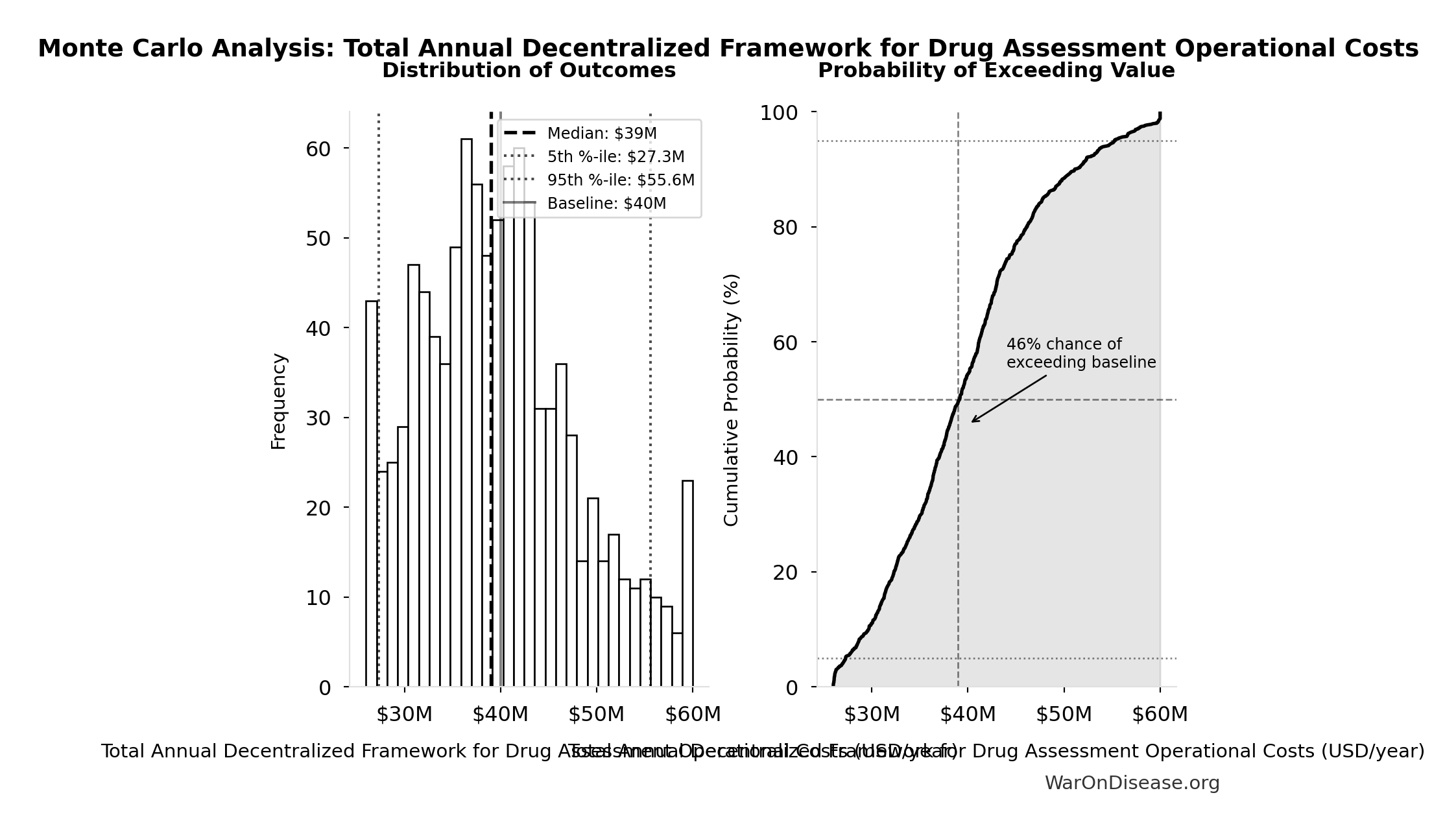
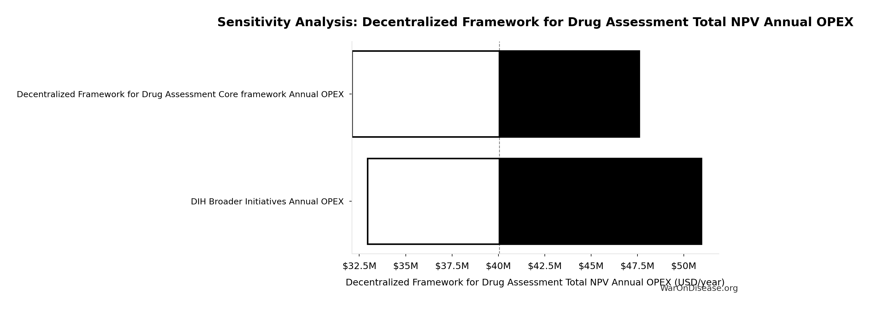
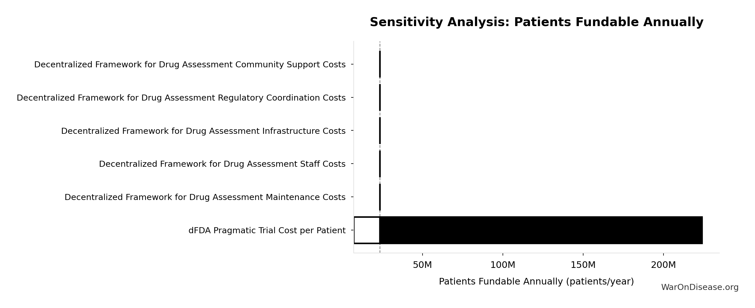
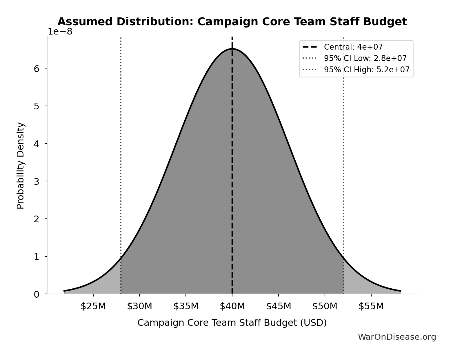
Total Annual Decentralized Framework for Drug Assessment Operational Costs: $40M
Total annual Decentralized Framework for Drug Assessment operational costs (sum of all components: platform + staff + infra + regulatory + community)
Inputs:
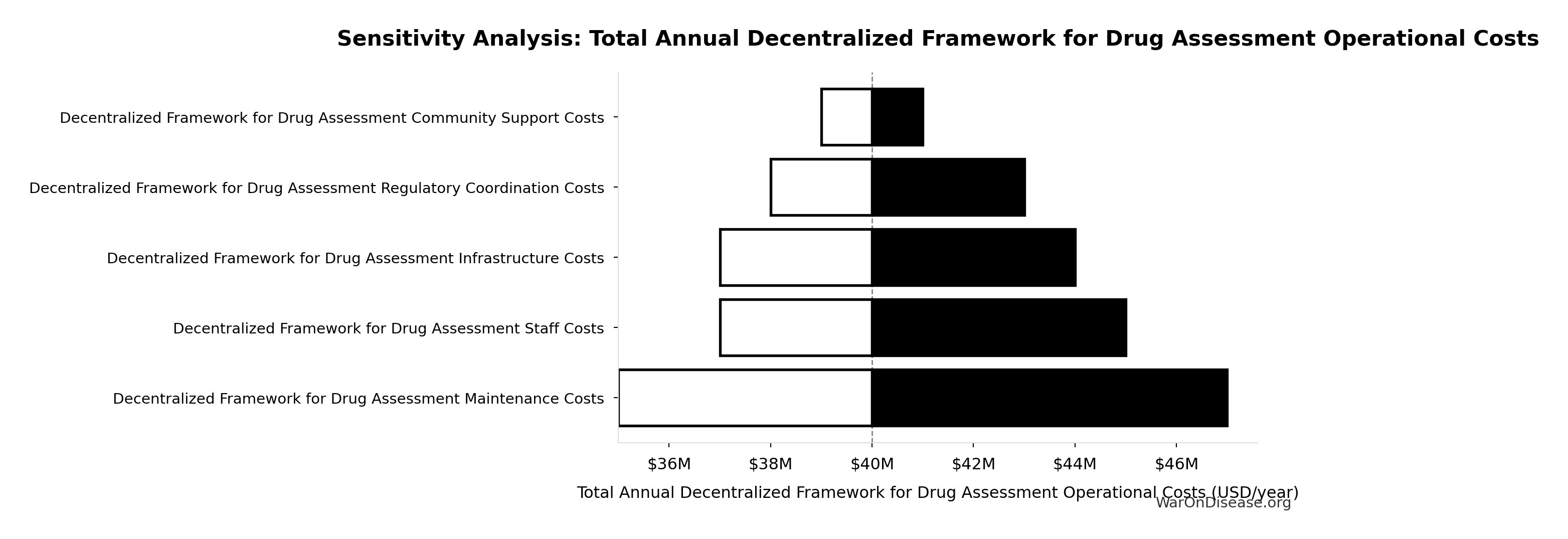
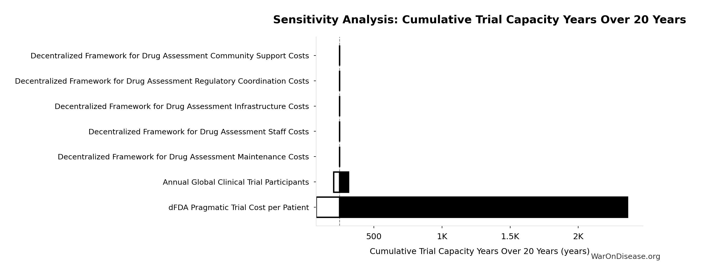
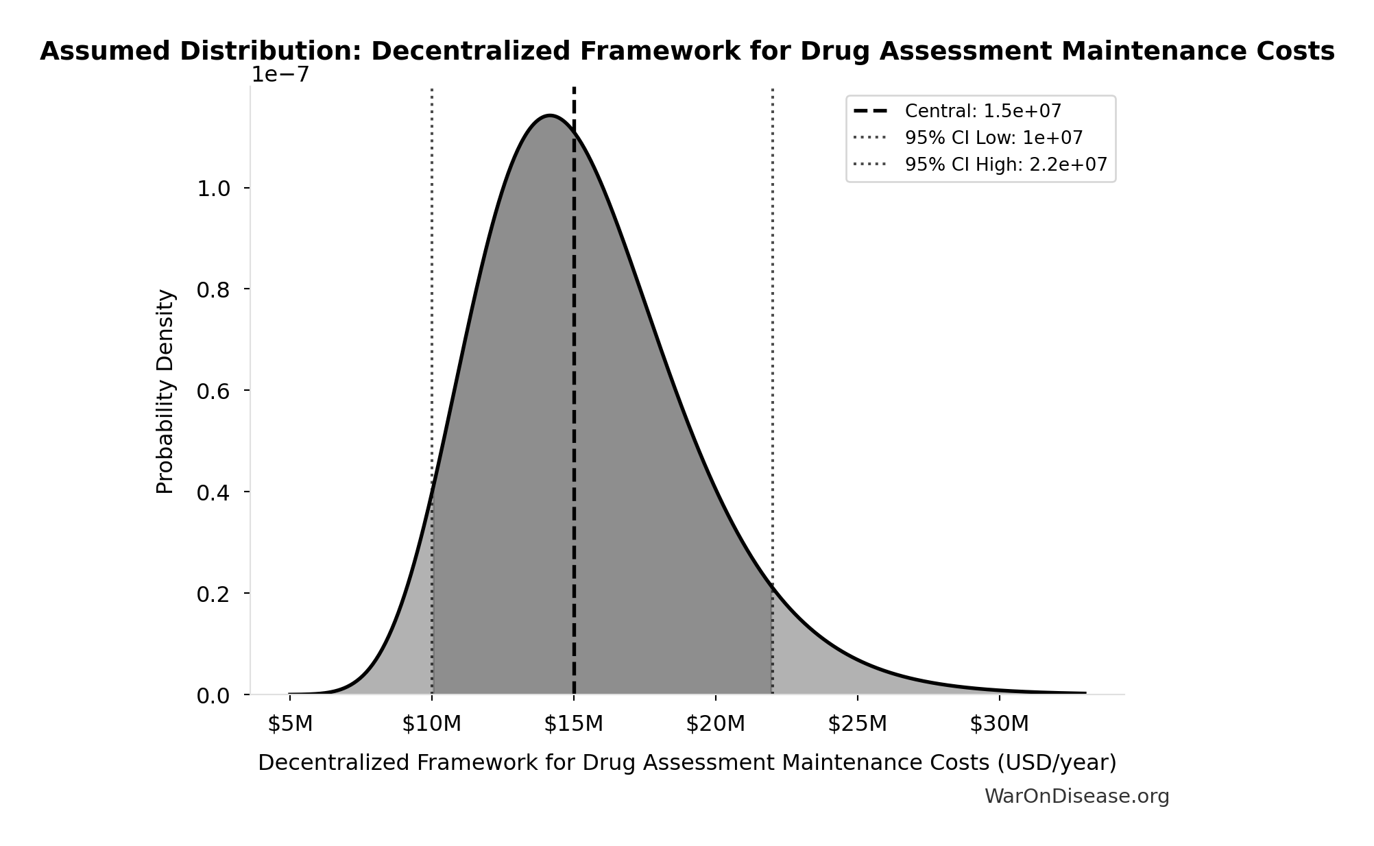
- Decentralized Framework for Drug Assessment Maintenance Costs: $15M (95% CI: $10M - $22M)
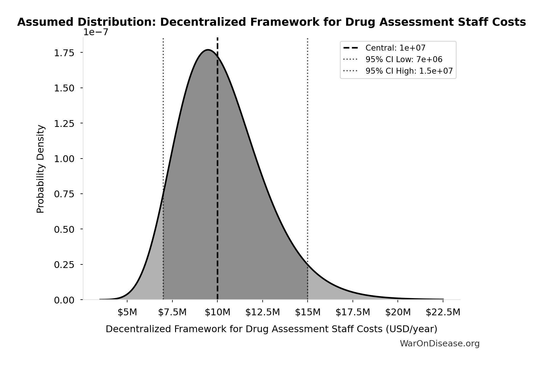
- Decentralized Framework for Drug Assessment Staff Costs: $10M (95% CI: $7M - $15M)
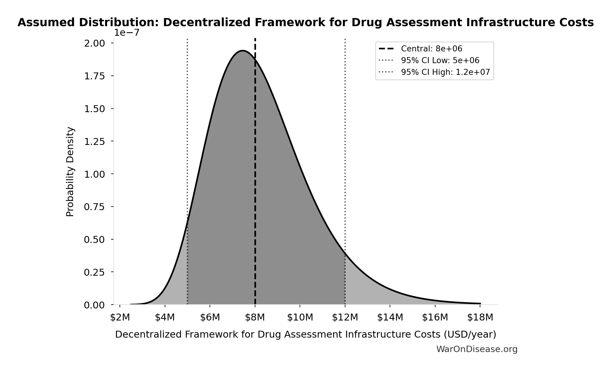
- Decentralized Framework for Drug Assessment Infrastructure Costs: $8M (95% CI: $5M - $12M)
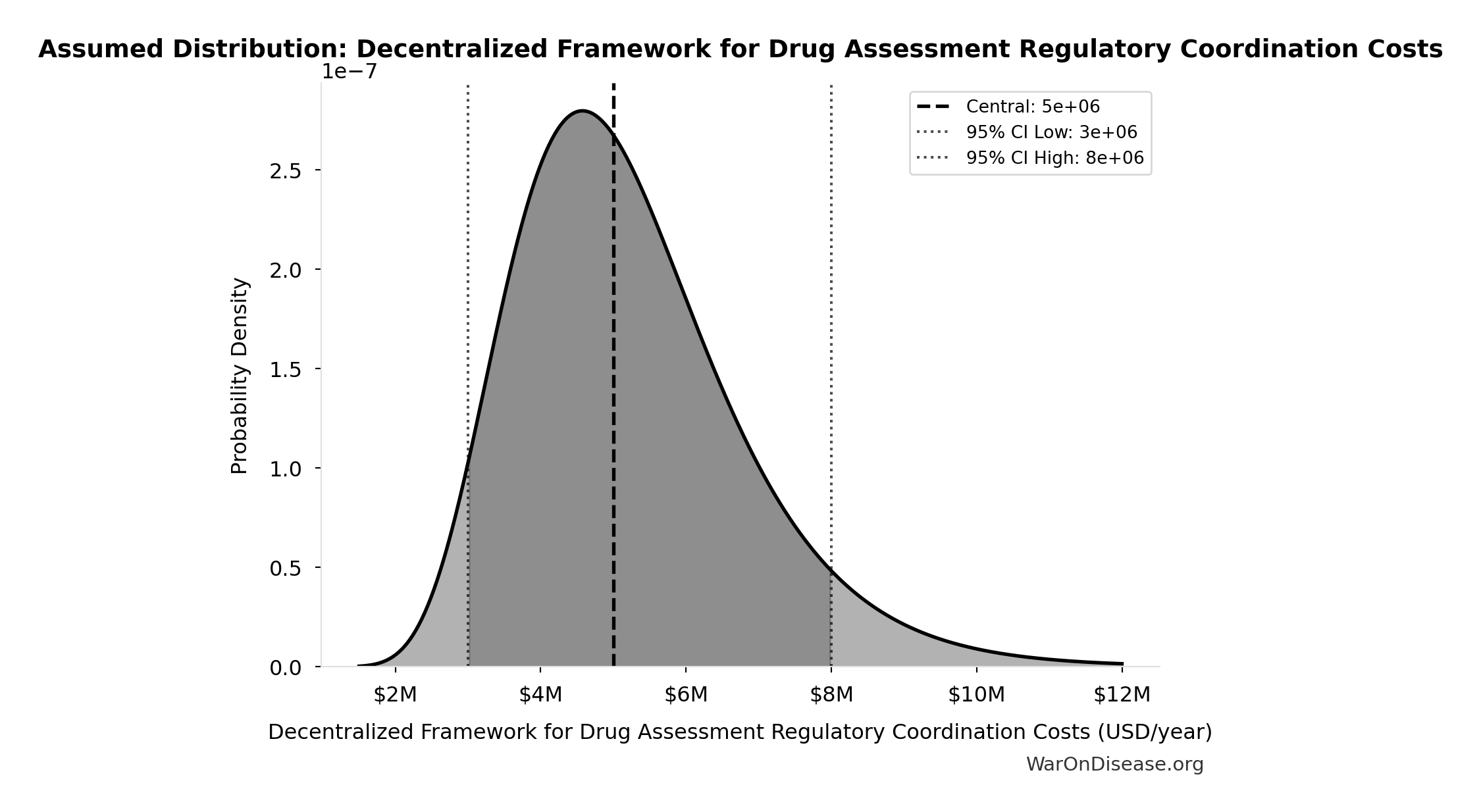
- Decentralized Framework for Drug Assessment Regulatory Coordination Costs: $5M (95% CI: $3M - $8M)
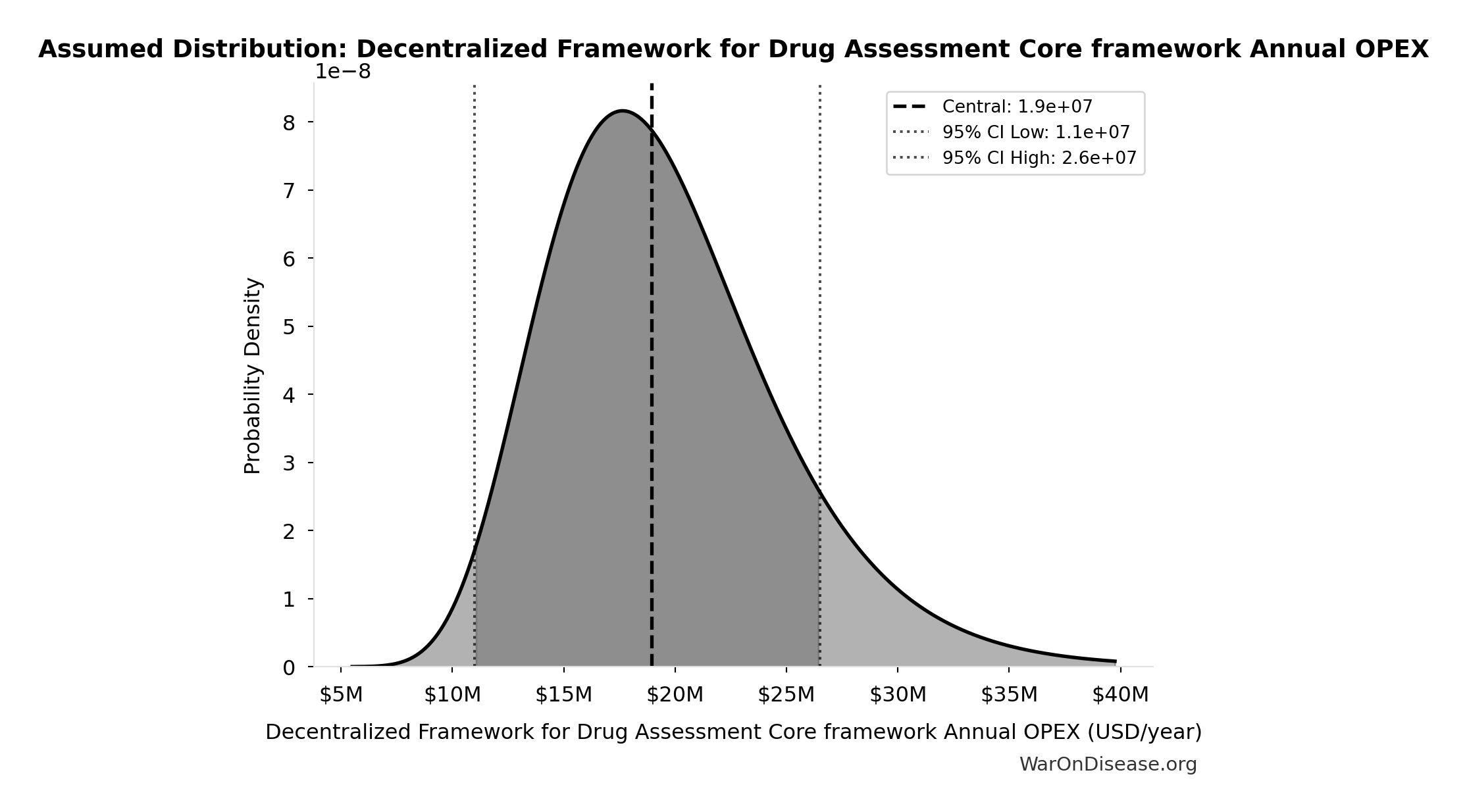
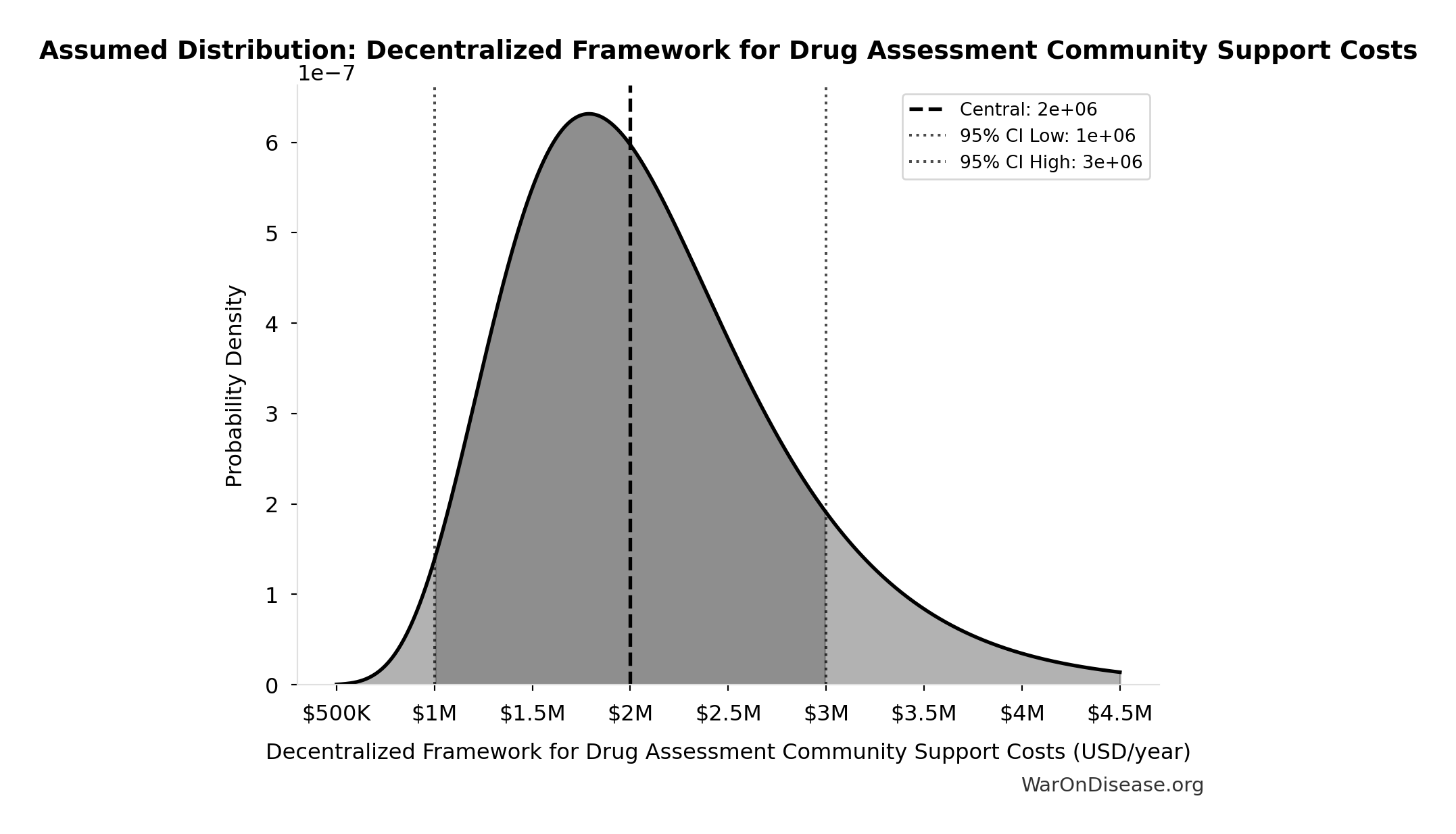
- Decentralized Framework for Drug Assessment Community Support Costs: $2M (95% CI: $1M - $3M)
\[ \begin{gathered} OPEX_{dFDA} \\ = Cost_{platform} + Cost_{staff} + Cost_{infra} \\ + Cost_{regulatory} + Cost_{community} \\ = \$15M + \$10M + \$8M + \$5M + \$2M \\ = \$40M \end{gathered} \]
✓ High confidence
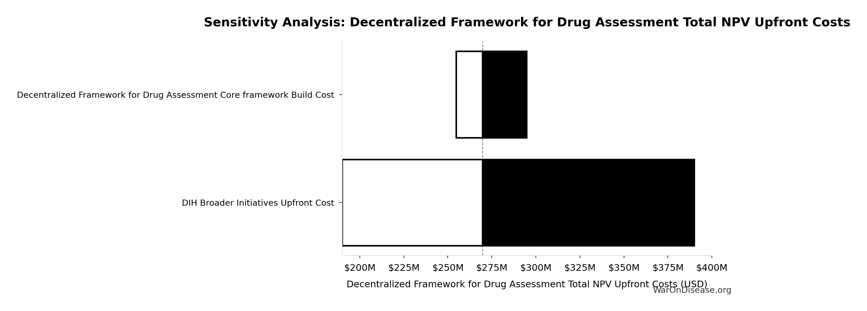
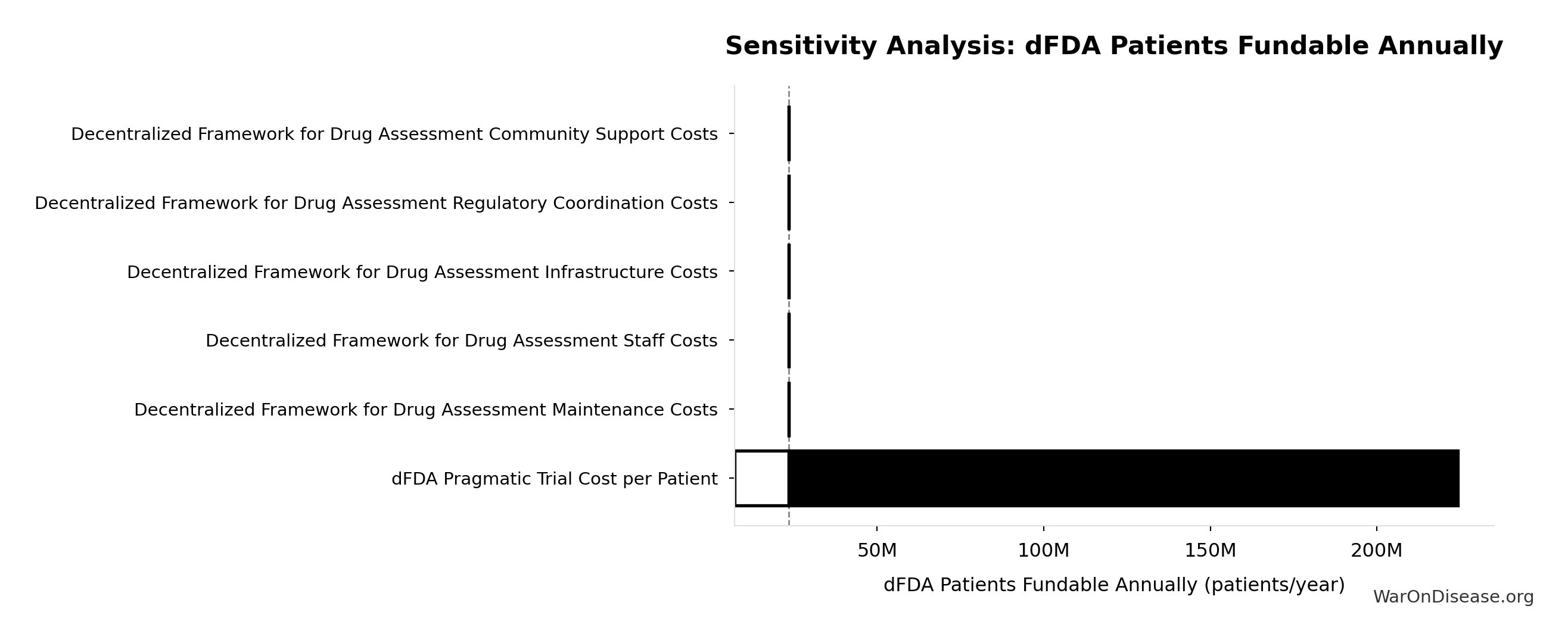
Sensitivity Analysis
Sensitivity Indices for Total Annual Decentralized Framework for Drug Assessment Operational Costs
Regression-based sensitivity showing which inputs explain the most variance in the output.
| Input Parameter | Sensitivity Coefficient | Interpretation |
|---|---|---|
| Decentralized Framework for Drug Assessment Maintenance Costs (USD/year) | 0.3542 | Moderate driver |
| Decentralized Framework for Drug Assessment Staff Costs (USD/year) | 0.2355 | Weak driver |
| Decentralized Framework for Drug Assessment Infrastructure Costs (USD/year) | 0.2060 | Weak driver |
| Decentralized Framework for Drug Assessment Regulatory Coordination Costs (USD/year) | 0.1469 | Weak driver |
| Decentralized Framework for Drug Assessment Community Support Costs (USD/year) | 0.0576 | Minimal effect |
Interpretation: Standardized coefficients show the change in output (in SD units) per 1 SD change in input. Values near ±1 indicate strong influence; values exceeding ±1 may occur with correlated inputs.
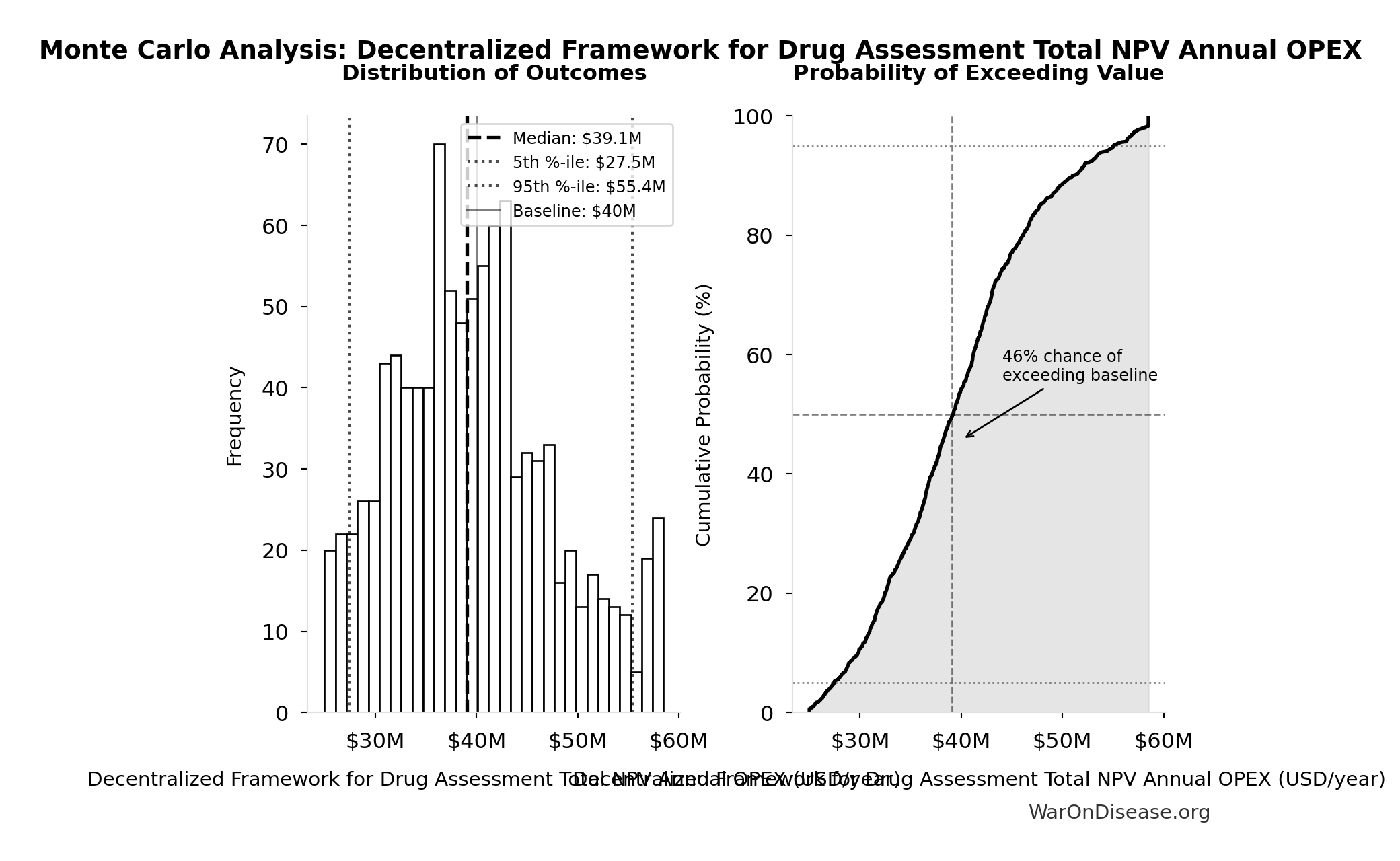
Monte Carlo Distribution
Simulation Results Summary: Total Annual Decentralized Framework for Drug Assessment Operational Costs
| Statistic | Value |
|---|---|
| Baseline (deterministic) | $40M |
| Mean (expected value) | $39.9M |
| Median (50th percentile) | $39M |
| Standard Deviation | $8.21M |
| 90% Range (5th-95th percentile) | [$27.3M, $55.6M] |
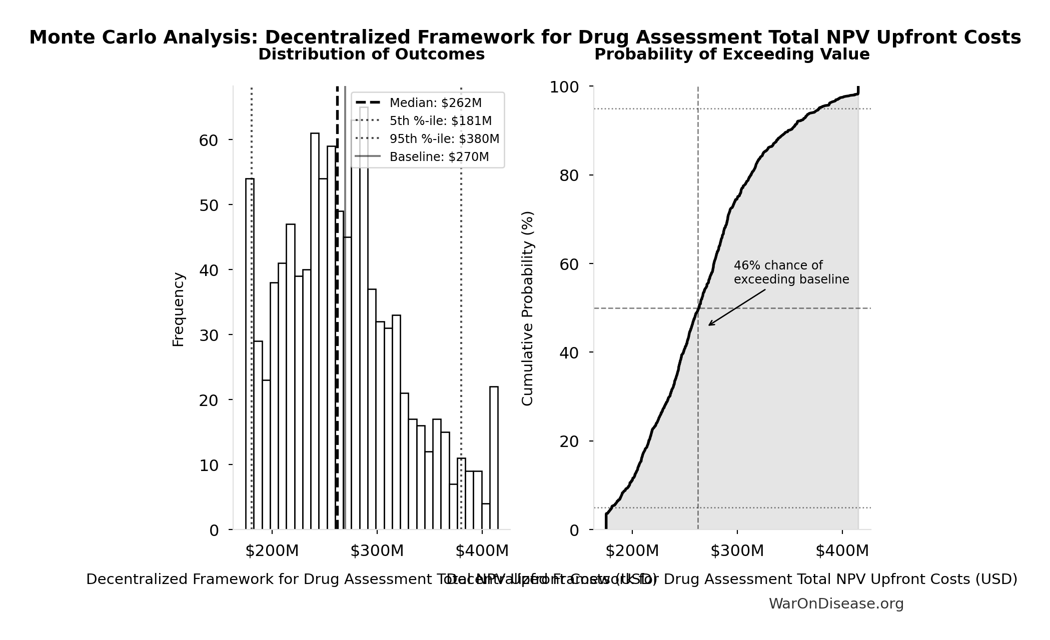
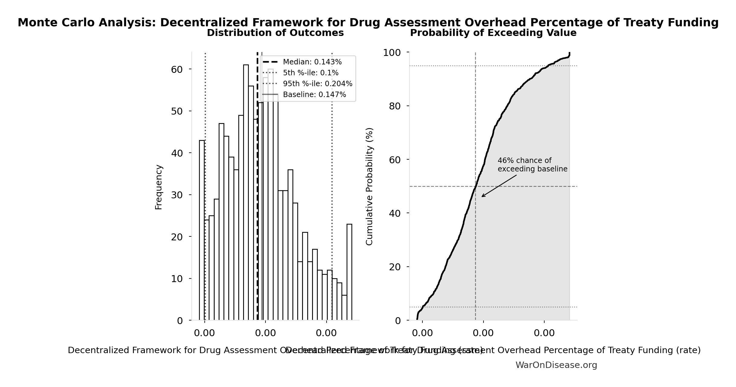
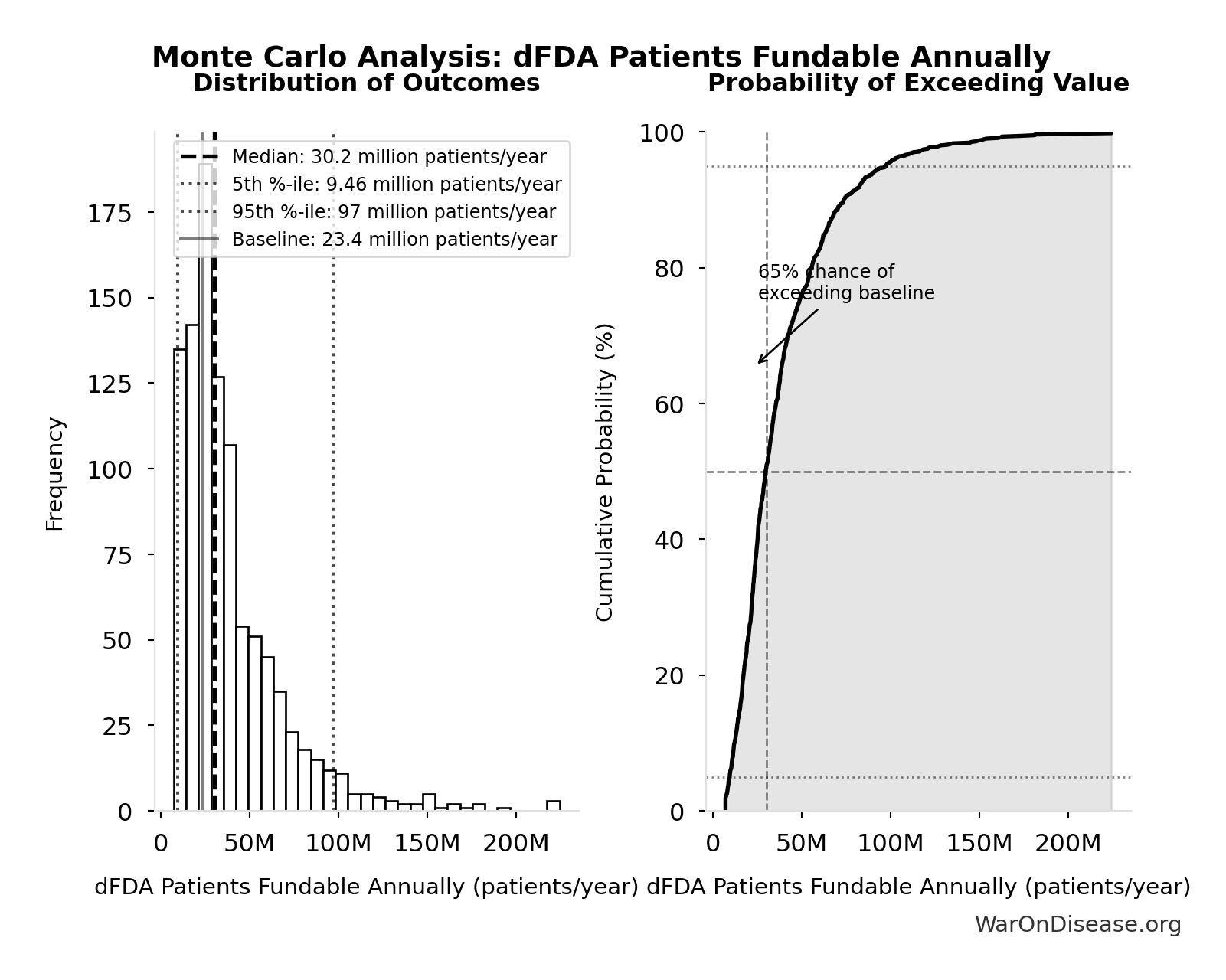
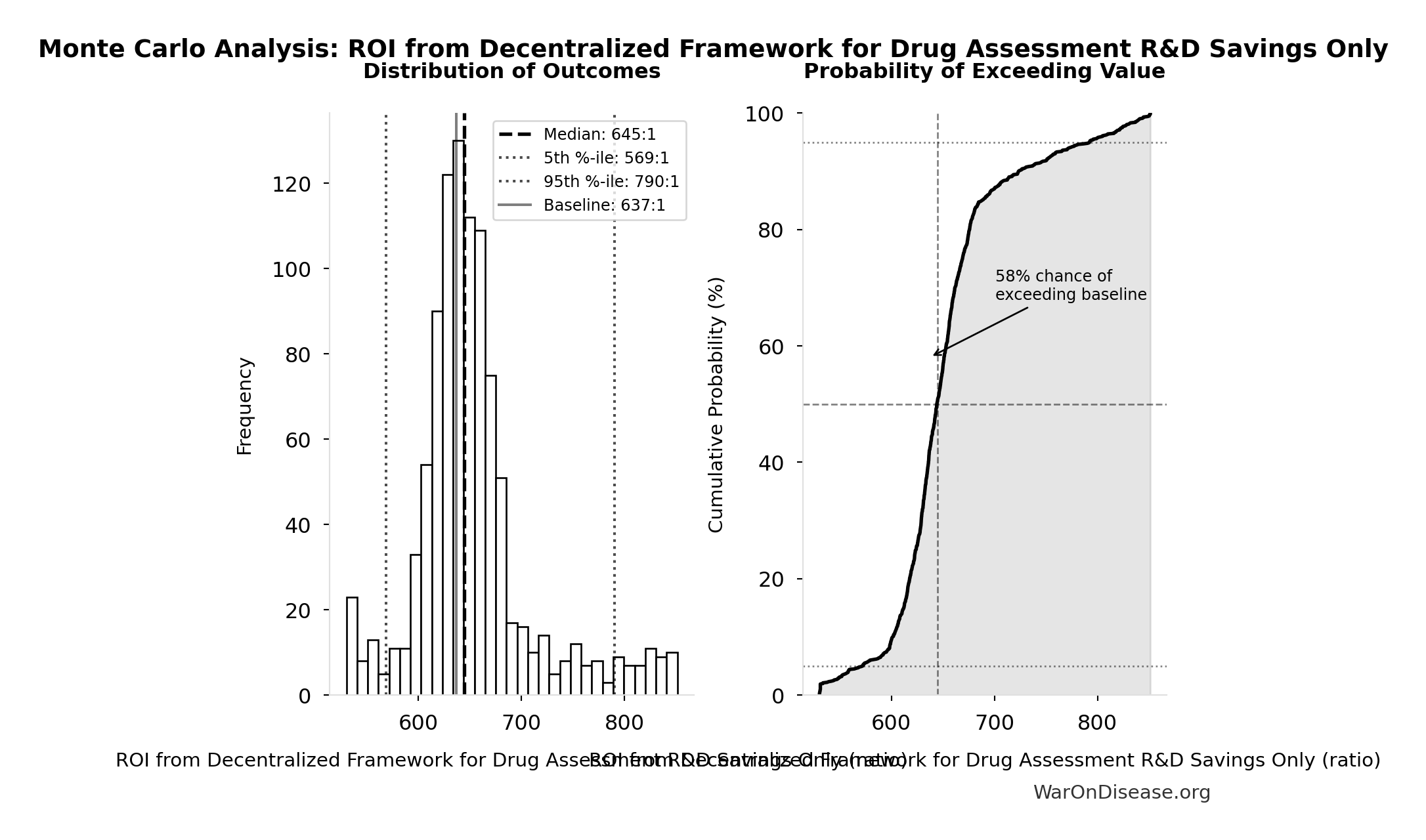
The histogram shows the distribution of Total Annual Decentralized Framework for Drug Assessment Operational Costs across 10,000 Monte Carlo simulations. The CDF (right) shows the probability of the outcome exceeding any given value, which is useful for risk assessment.
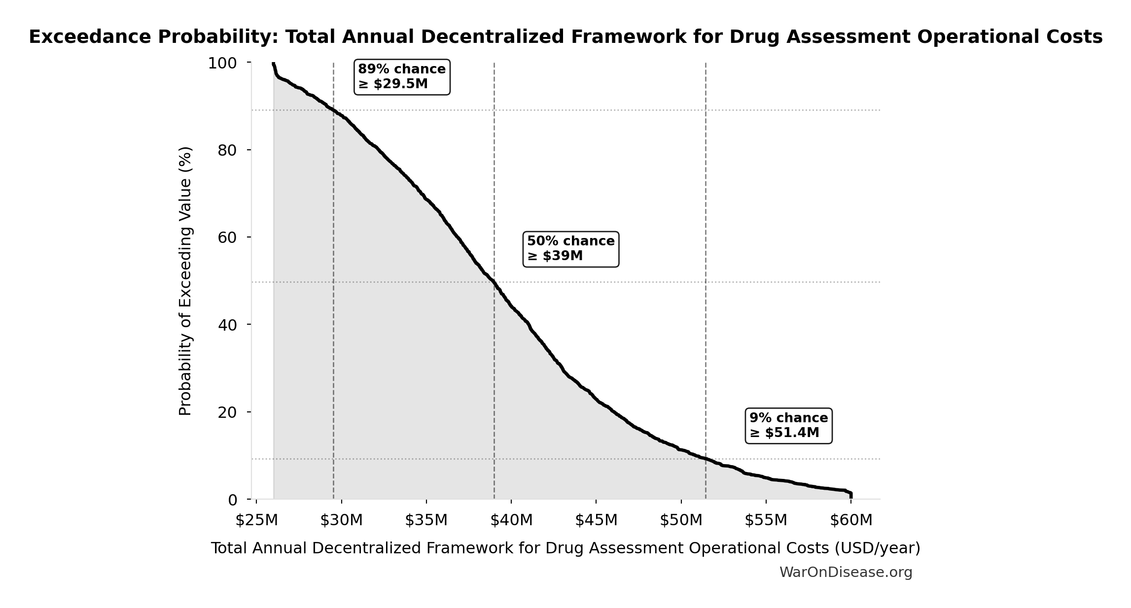
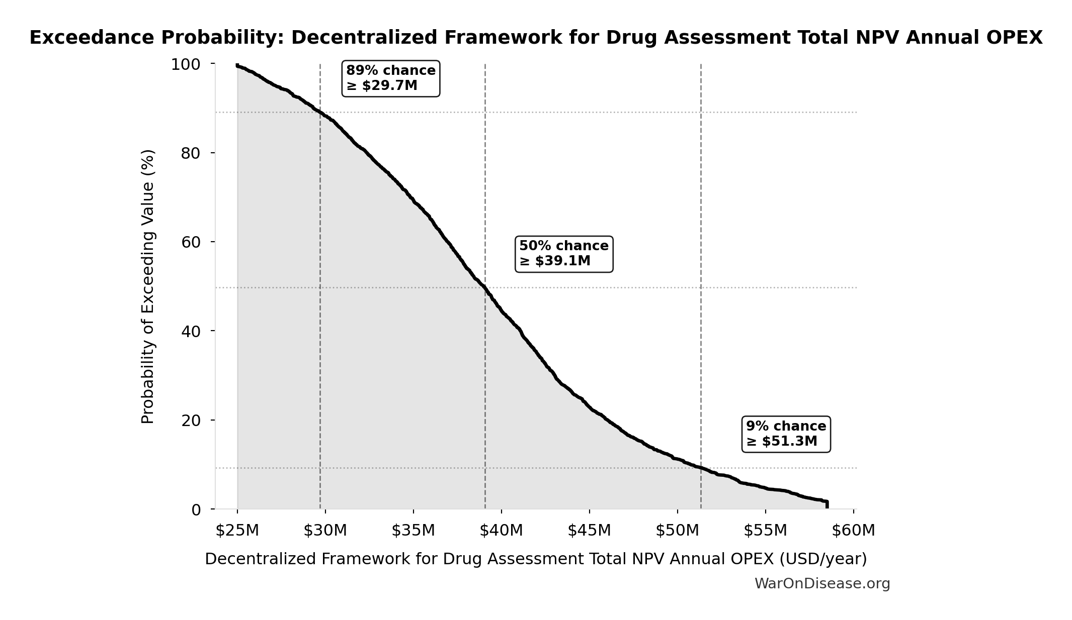
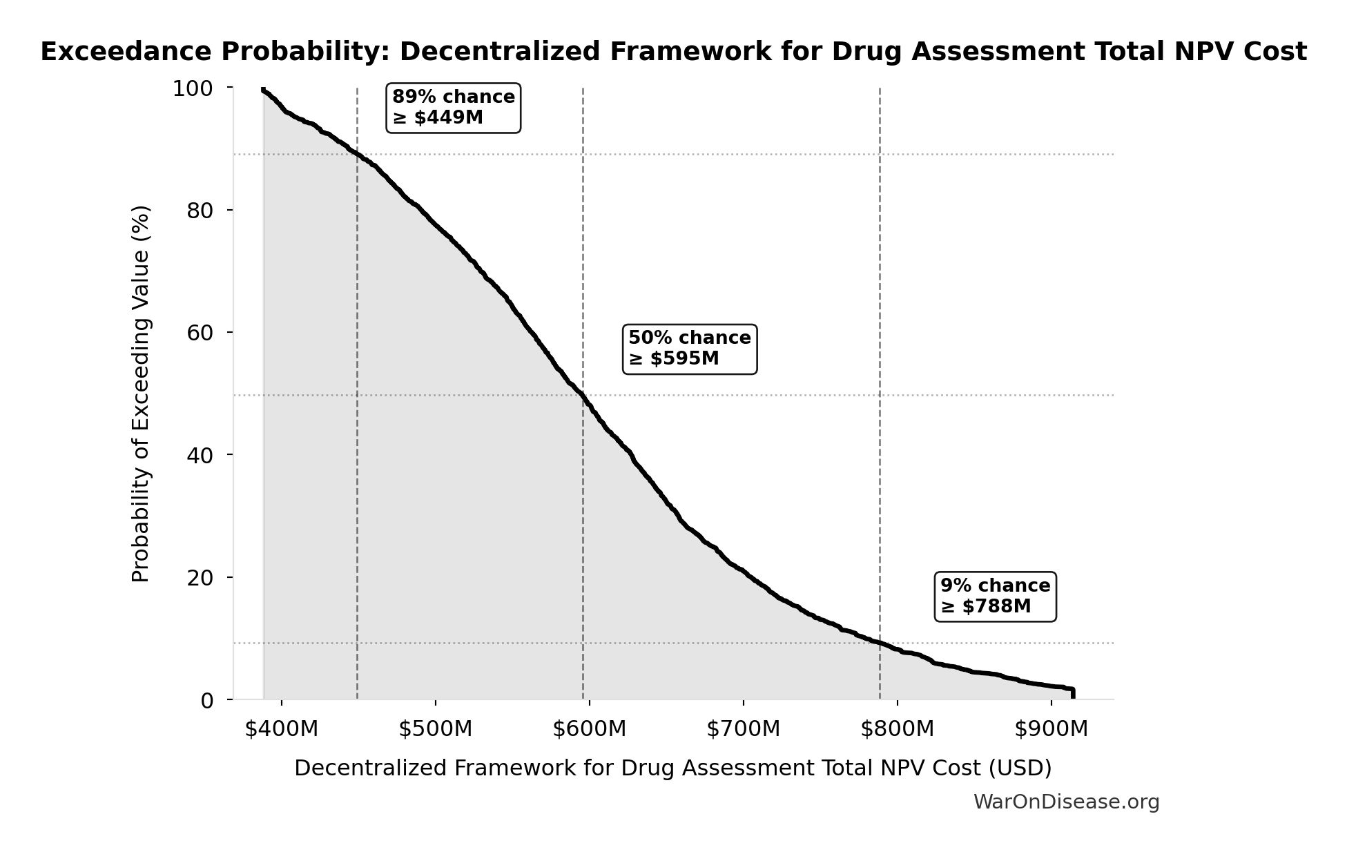
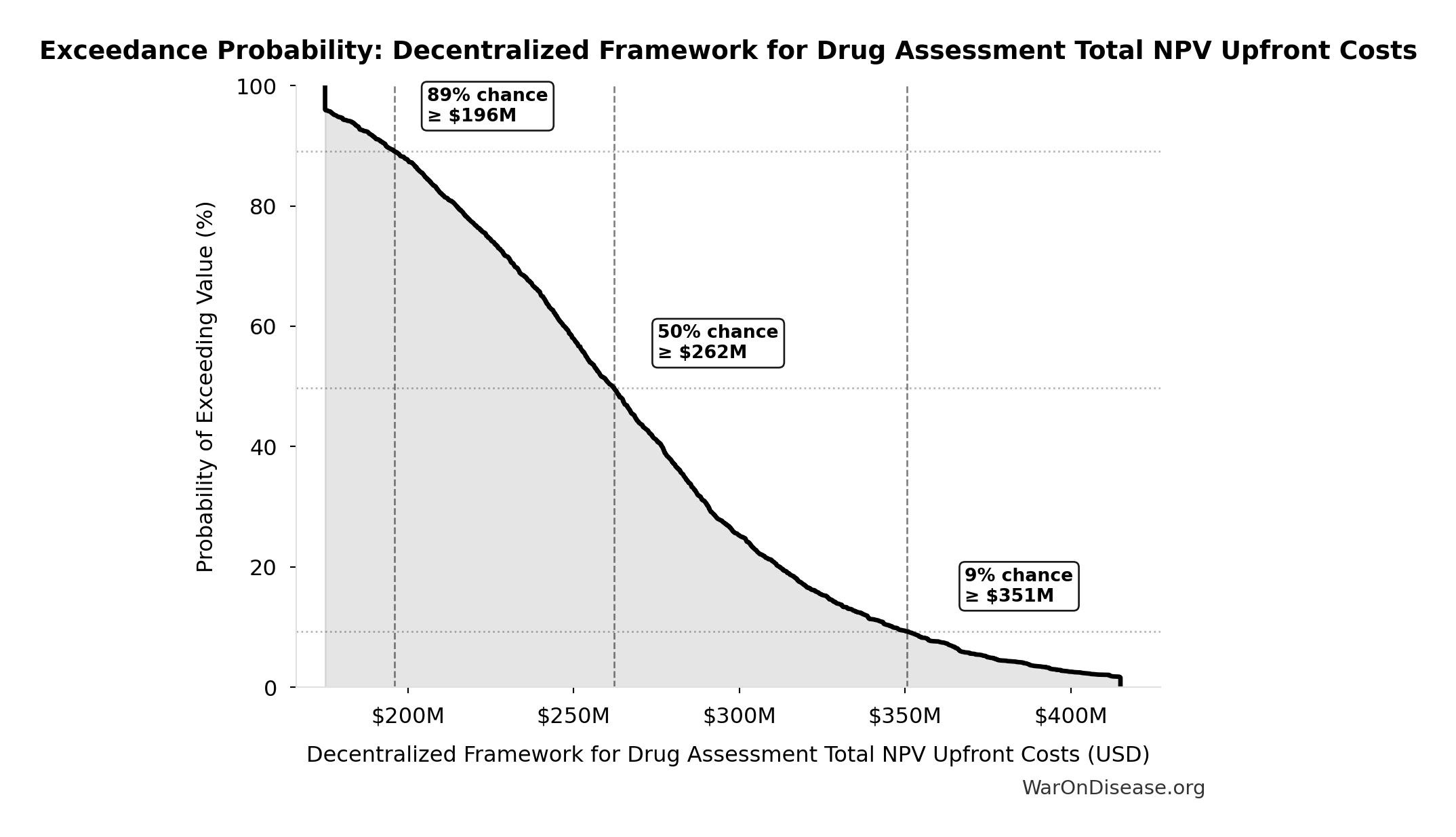
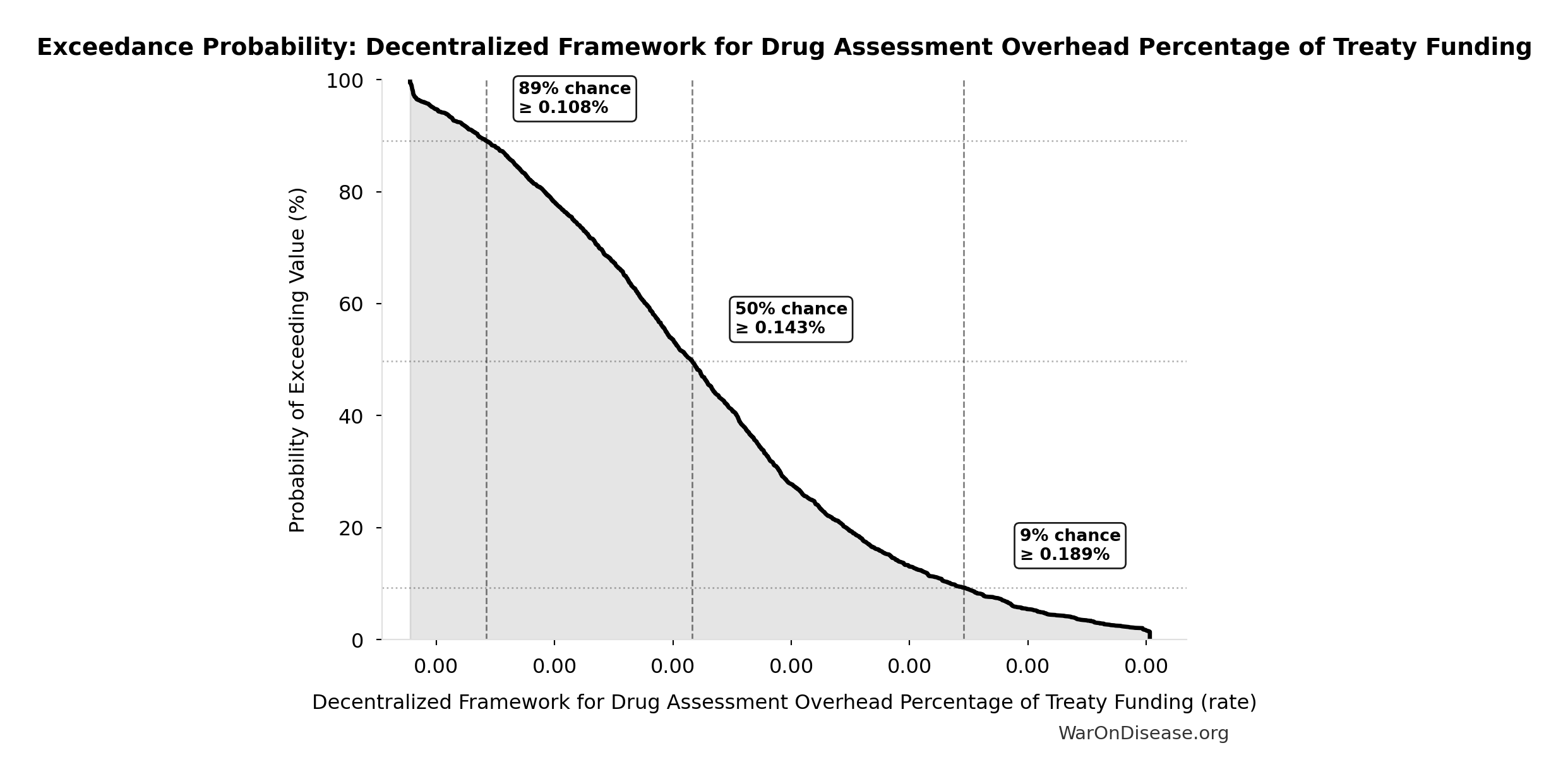
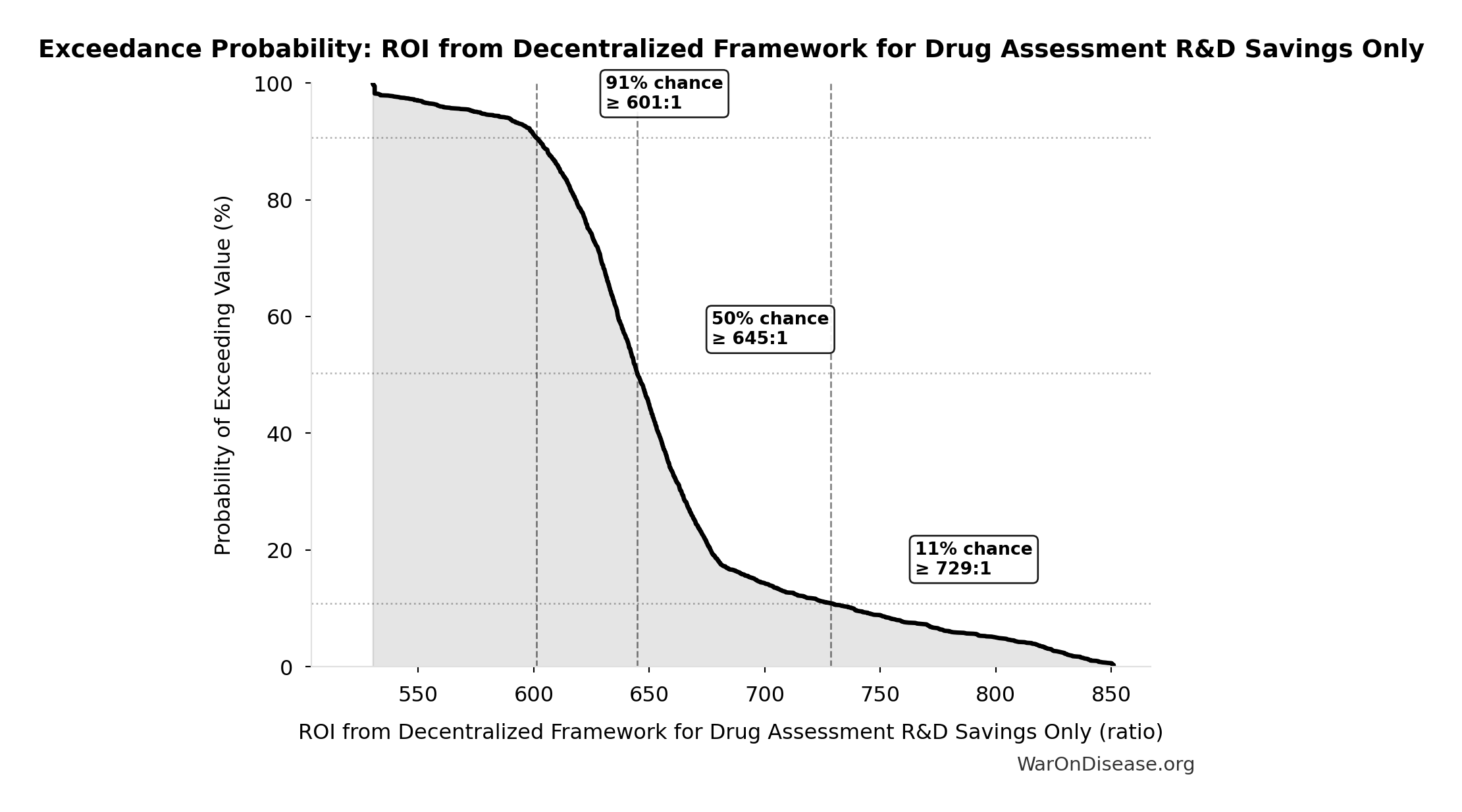
Exceedance Probability
This exceedance probability chart shows the likelihood that Total Annual Decentralized Framework for Drug Assessment Operational Costs will exceed any given threshold. Higher curves indicate more favorable outcomes with greater certainty.
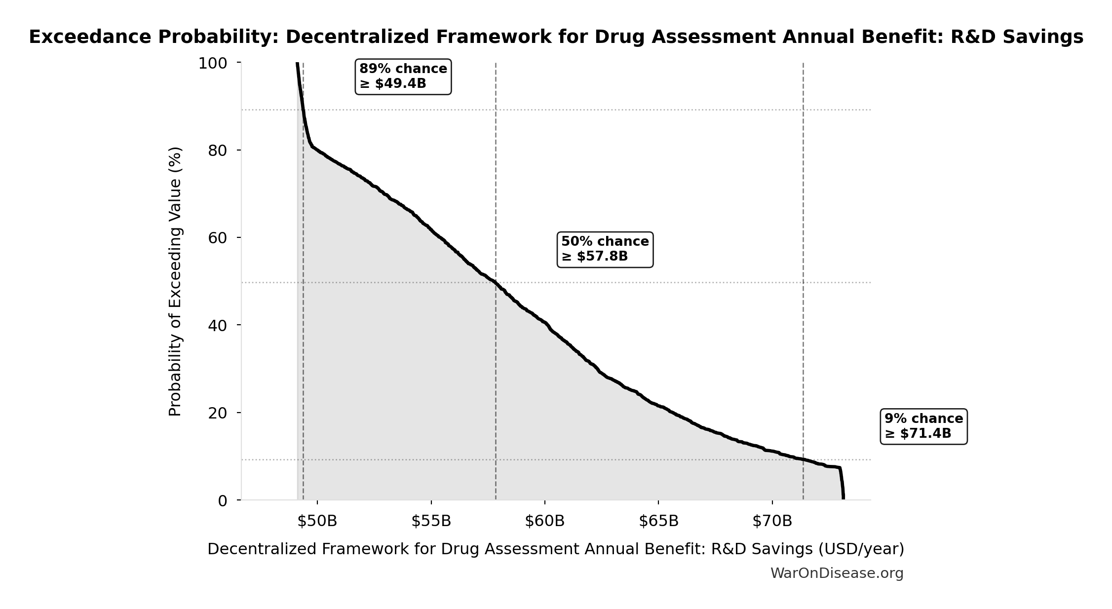
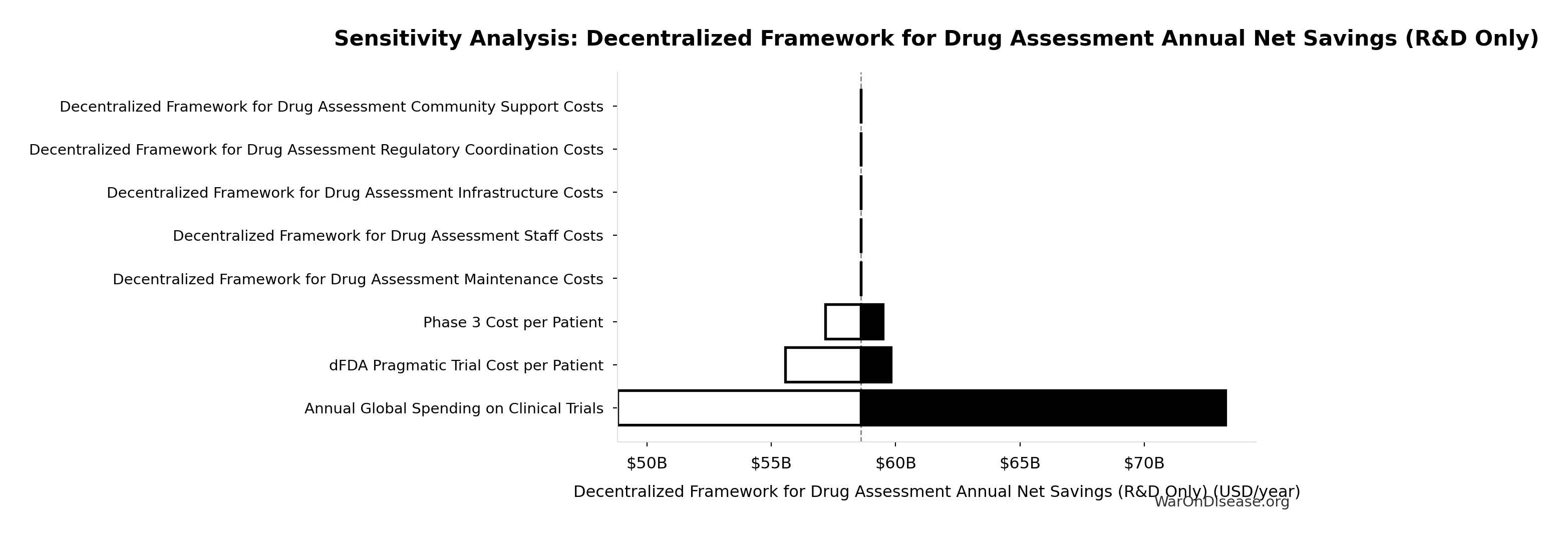
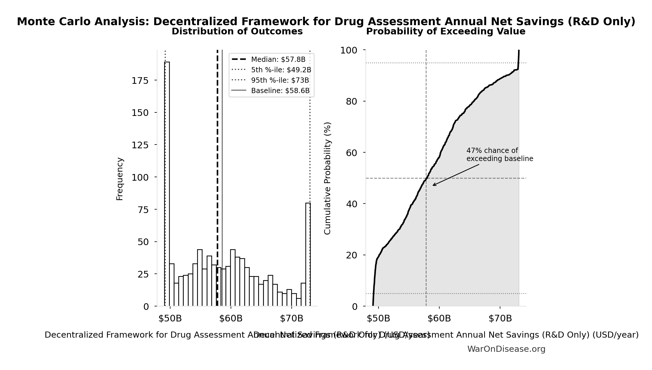
Decentralized Framework for Drug Assessment Annual Benefit: R&D Savings: $58.6B
Annual Decentralized Framework for Drug Assessment benefit from R&D savings (trial cost reduction, secondary component)
Inputs:
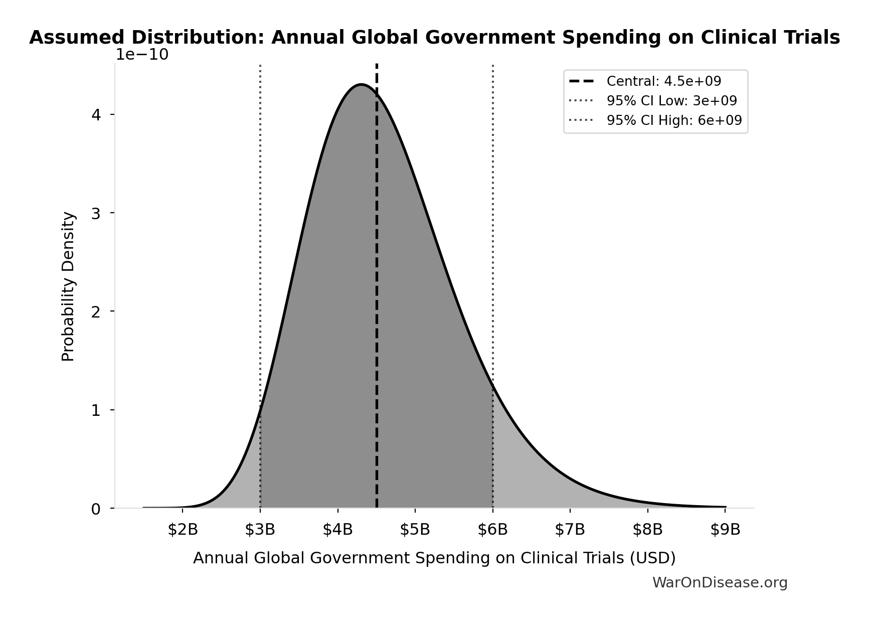
- Annual Global Spending on Clinical Trials 📊: $60B (95% CI: $50B - $75B)
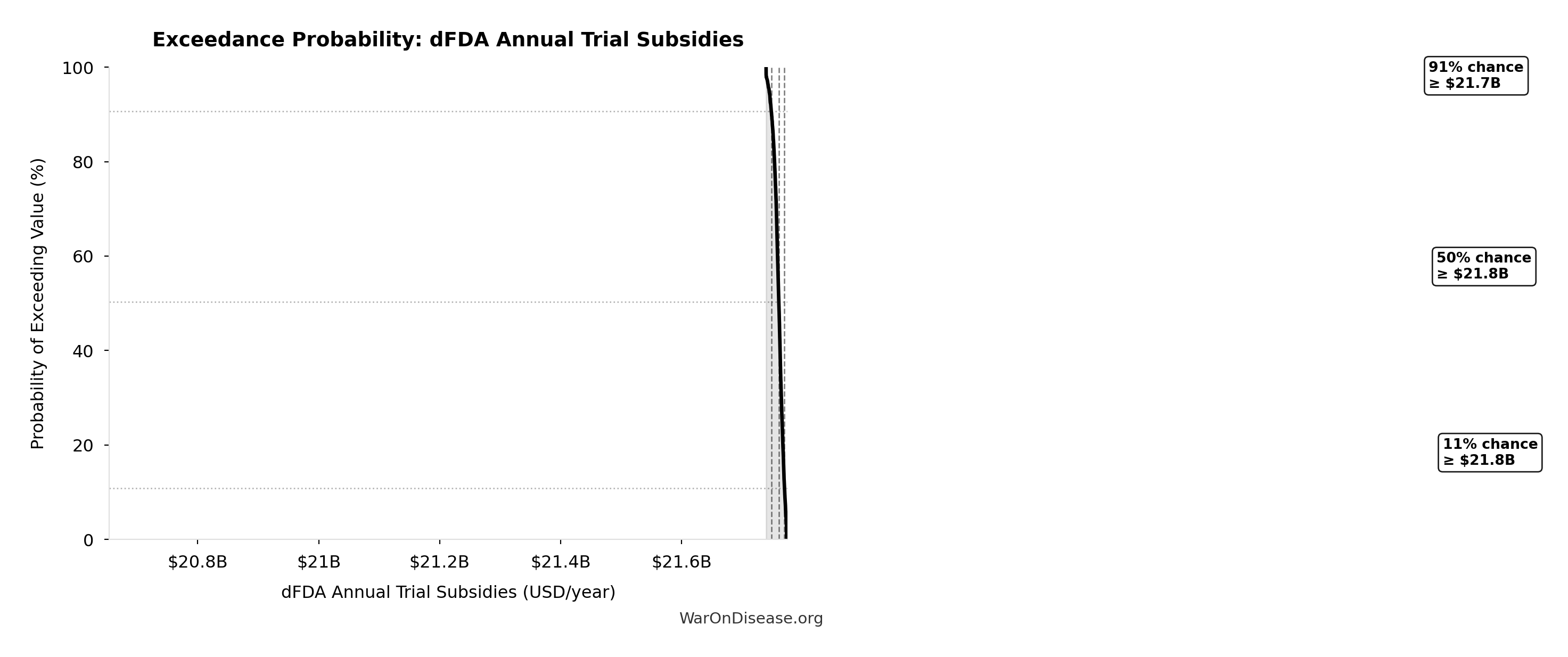
- dFDA Trial Cost Reduction Percentage 🔢: 97.7%
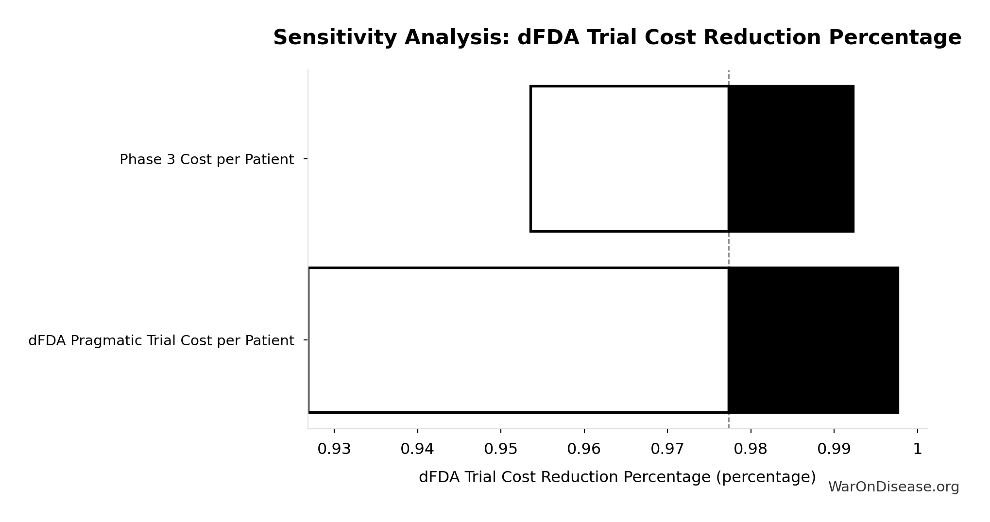
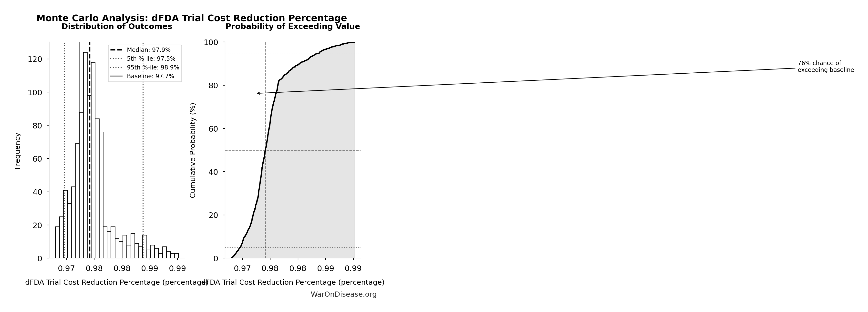
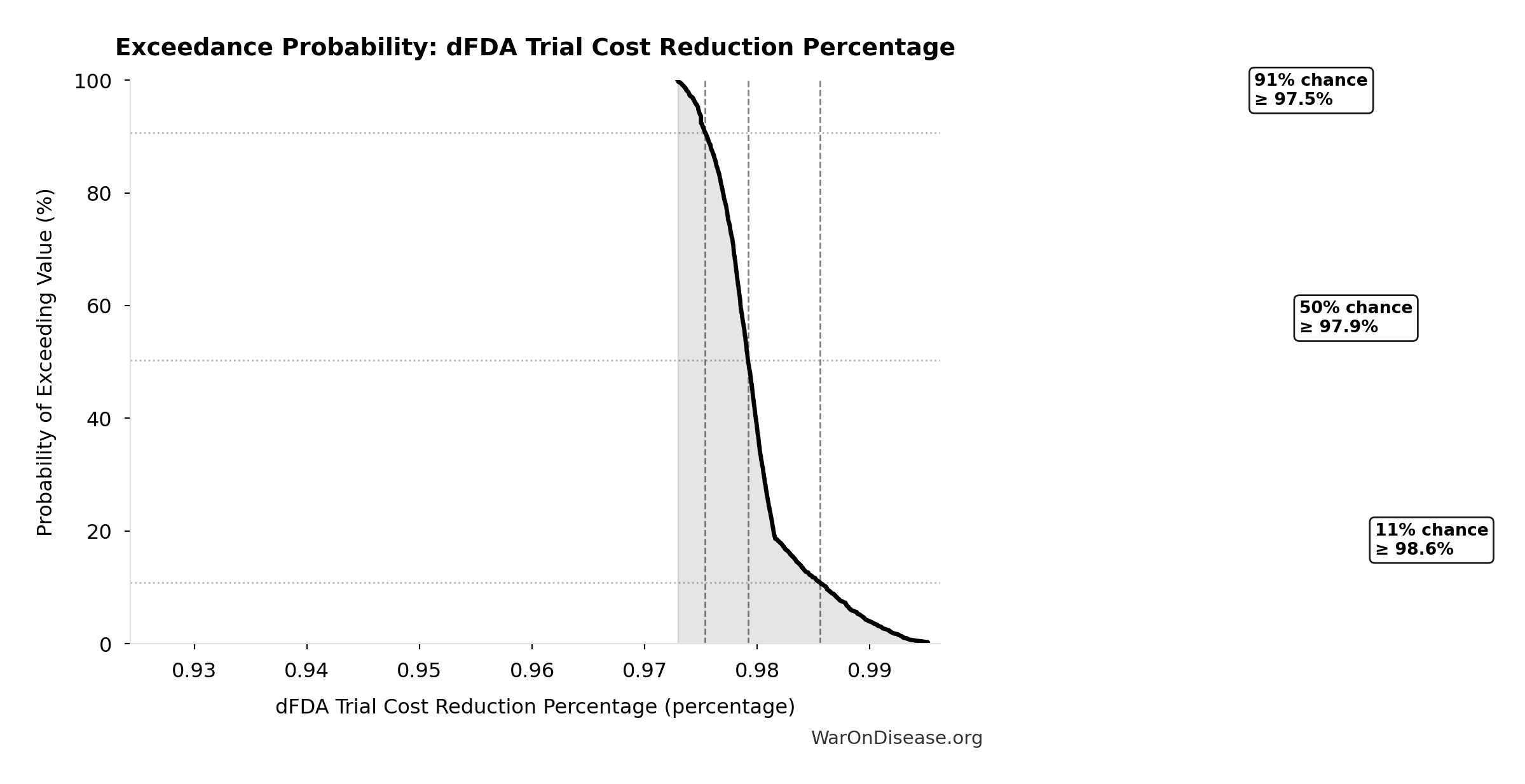
\[ \begin{gathered} Benefit_{RD,ann} \\ = Spending_{trials} \times Reduce_{pct} \\ = \$60B \times 97.7\% \\ = \$58.6B \end{gathered} \] where: \[ \begin{gathered} Reduce_{pct} \\ = 1 - \frac{Cost_{pragmatic,pt}}{Cost_{P3,pt}} \\ = 1 - \frac{\$929}{\$41K} \\ = 97.7\% \end{gathered} \] ✓ High confidence
Sensitivity Analysis
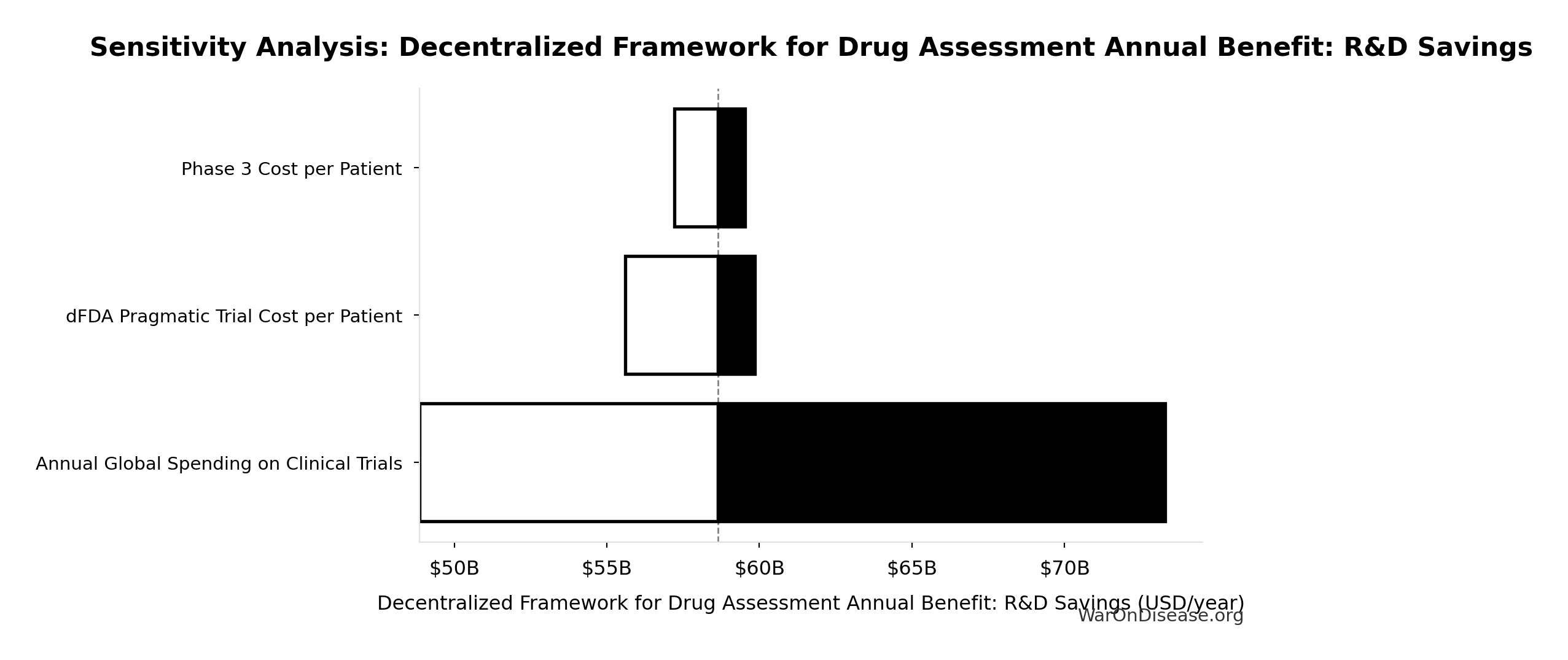
Sensitivity Indices for Decentralized Framework for Drug Assessment Annual Benefit: R&D Savings
Regression-based sensitivity showing which inputs explain the most variance in the output.
| Input Parameter | Sensitivity Coefficient | Interpretation |
|---|---|---|
| Annual Global Spending on Clinical Trials (USD) | 1.0205 | Strong driver |
| dFDA Trial Cost Reduction Percentage (percentage) | 0.0244 | Minimal effect |
Interpretation: Standardized coefficients show the change in output (in SD units) per 1 SD change in input. Values near ±1 indicate strong influence; values exceeding ±1 may occur with correlated inputs.
Monte Carlo Distribution
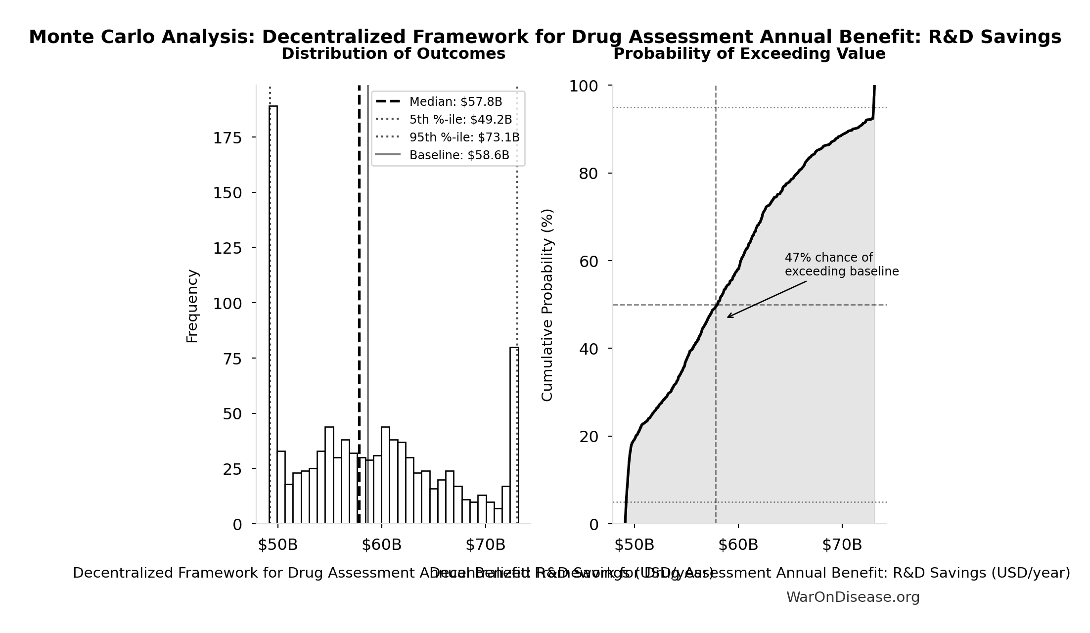
Simulation Results Summary: Decentralized Framework for Drug Assessment Annual Benefit: R&D Savings
| Statistic | Value |
|---|---|
| Baseline (deterministic) | $58.6B |
| Mean (expected value) | $58.8B |
| Median (50th percentile) | $57.8B |
| Standard Deviation | $7.66B |
| 90% Range (5th-95th percentile) | [$49.2B, $73.1B] |
The histogram shows the distribution of Decentralized Framework for Drug Assessment Annual Benefit: R&D Savings across 10,000 Monte Carlo simulations. The CDF (right) shows the probability of the outcome exceeding any given value, which is useful for risk assessment.
Exceedance Probability
This exceedance probability chart shows the likelihood that Decentralized Framework for Drug Assessment Annual Benefit: R&D Savings will exceed any given threshold. Higher curves indicate more favorable outcomes with greater certainty.
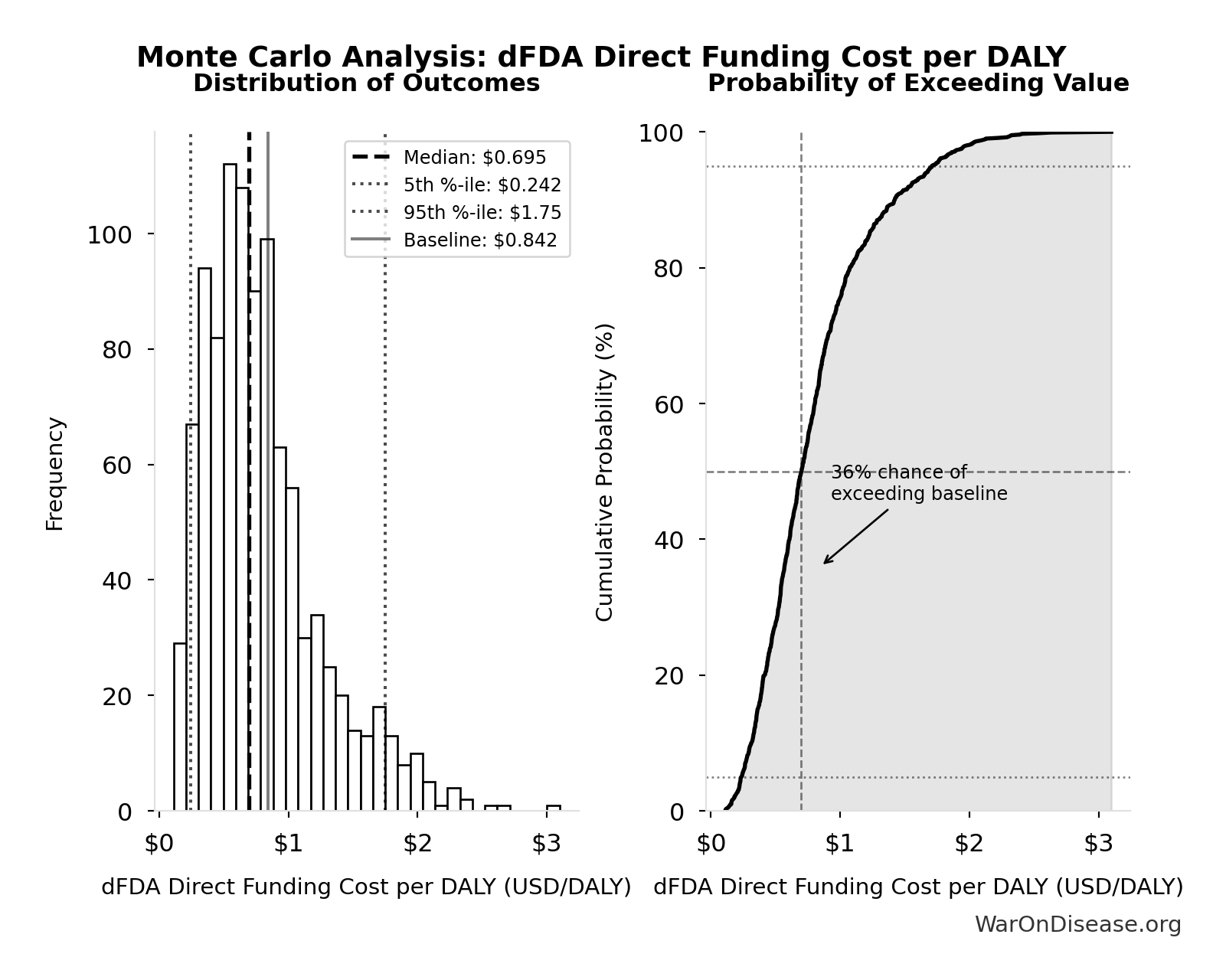
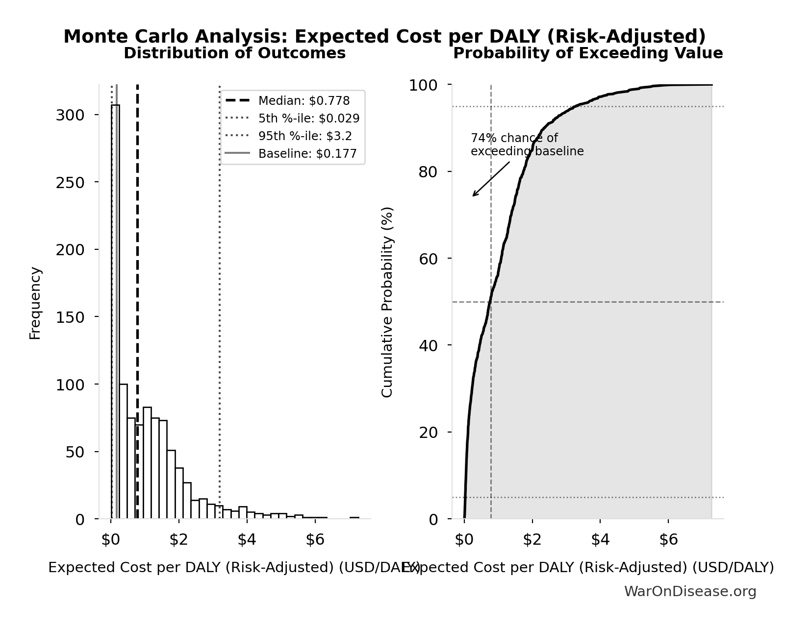
dFDA Direct Funding Cost per DALY: $0.842
Cost per DALY at direct funding level for the therapeutic space exploration period. Still highly cost-effective vs bed nets.
Inputs:
- dFDA Direct Funding NPV (Exploration Period) 🔢: $476B
- Total DALYs from Elimination of Efficacy Lag Plus Earlier Treatment Discovery from Higher Trial Throughput 🔢: 565 billion DALYs
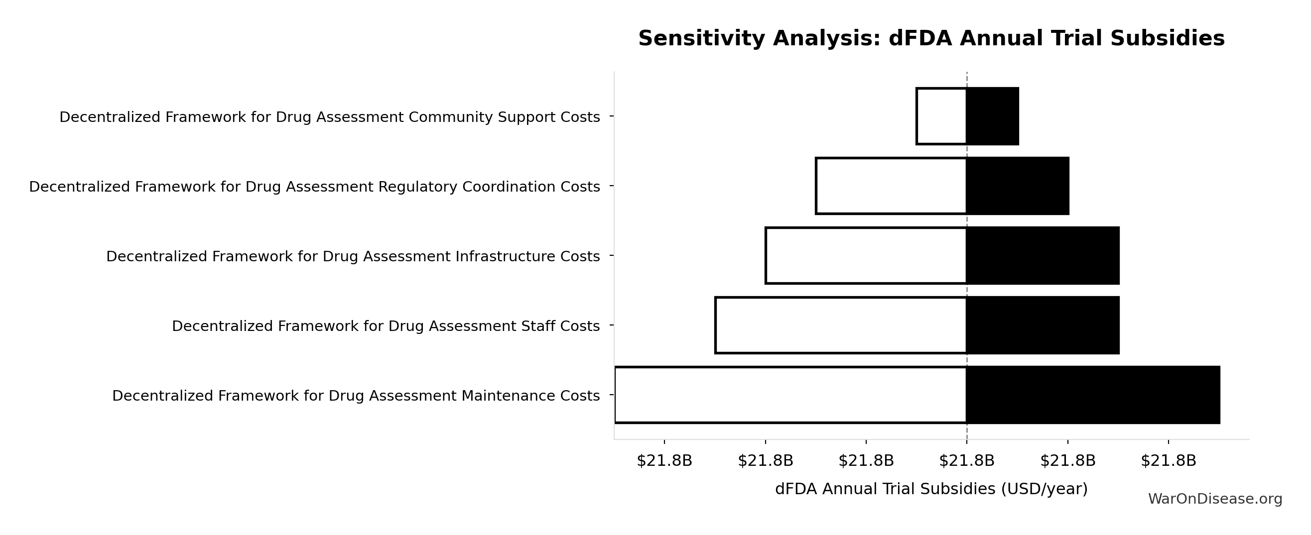
\[ \begin{gathered} Cost_{direct,DALY} \\ = \frac{NPV_{direct}}{DALYs_{max}} \\ = \frac{\$476B}{565B} \\ = \$0.842 \end{gathered} \] where: \[ NPV_{direct} = Funding_{ann} \times \frac{1 - (1+r)^{-T}}{r} \] where: \[ \begin{gathered} T_{queue,dFDA} \\ = \frac{T_{queue,SQ}}{k_{capacity}} \\ = \frac{443}{12.3} \\ = 36 \end{gathered} \] where: \[ \begin{gathered} T_{queue,SQ} \\ = \frac{N_{untreated}}{Treatments_{new,ann}} \\ = \frac{6{,}650}{15} \\ = 443 \end{gathered} \] where: \[ \begin{gathered} N_{untreated} \\ = N_{rare} \times 0.95 \\ = 7{,}000 \times 0.95 \\ = 6{,}650 \end{gathered} \] where: \[ \begin{gathered} k_{capacity} \\ = \frac{N_{fundable,dFDA}}{Slots_{curr}} \\ = \frac{23.4M}{1.9M} \\ = 12.3 \end{gathered} \] where: \[ \begin{gathered} N_{fundable,dFDA} \\ = \frac{Subsidies_{dFDA,ann}}{Cost_{pragmatic,pt}} \\ = \frac{\$21.8B}{\$929} \\ = 23.4M \end{gathered} \] where: \[ \begin{gathered} Subsidies_{dFDA,ann} \\ = Funding_{dFDA,ann} - OPEX_{dFDA} \\ = \$21.8B - \$40M \\ = \$21.8B \end{gathered} \] where: \[ \begin{gathered} OPEX_{dFDA} \\ = Cost_{platform} + Cost_{staff} + Cost_{infra} \\ + Cost_{regulatory} + Cost_{community} \\ = \$15M + \$10M + \$8M + \$5M + \$2M \\ = \$40M \end{gathered} \] where: \[ \begin{gathered} DALYs_{max} \\ = DALYs_{global,ann} \times Pct_{avoid,DALY} \times T_{accel,max} \\ = 2.88B \times 92.6\% \times 212 \\ = 565B \end{gathered} \] where: \[ T_{accel,max} = T_{accel} + T_{lag} = 204 + 8.2 = 212 \] where: \[ \begin{gathered} T_{accel} \\ = T_{first,SQ} \times \left(1 - \frac{1}{k_{capacity}}\right) \\ = 222 \times \left(1 - \frac{1}{12.3}\right) \\ = 204 \end{gathered} \] where: \[ \begin{gathered} T_{first,SQ} \\ = T_{queue,SQ} \times 0.5 \\ = 443 \times 0.5 \\ = 222 \end{gathered} \] ~ Medium confidence
Sensitivity Analysis
Sensitivity Indices for dFDA Direct Funding Cost per DALY
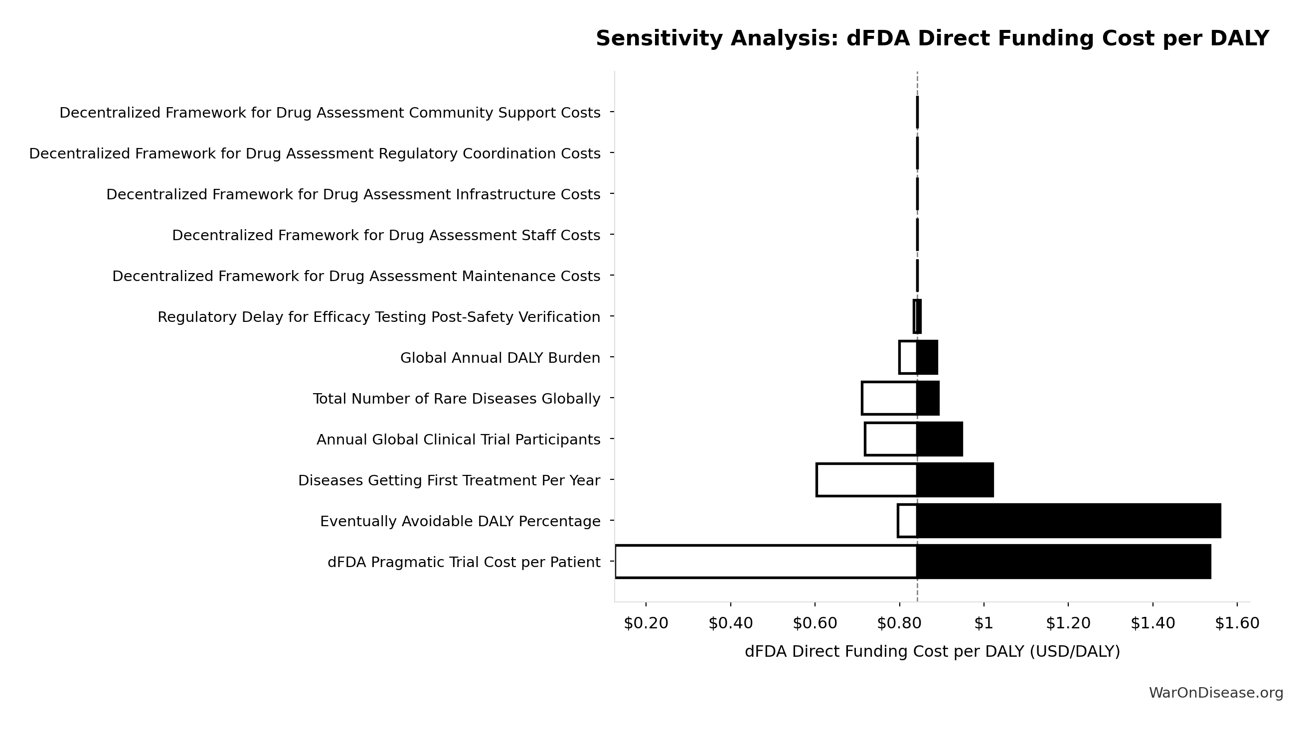
Regression-based sensitivity showing which inputs explain the most variance in the output.
| Input Parameter | Sensitivity Coefficient | Interpretation |
|---|---|---|
| Total DALYs from Elimination of Efficacy Lag Plus Earlier Treatment Discovery from Higher Trial Throughput (DALYs) | -0.5173 | Strong driver |
| dFDA Direct Funding NPV (Exploration Period) (USD) | 0.4592 | Moderate driver |
Interpretation: Standardized coefficients show the change in output (in SD units) per 1 SD change in input. Values near ±1 indicate strong influence; values exceeding ±1 may occur with correlated inputs.
Monte Carlo Distribution
Simulation Results Summary: dFDA Direct Funding Cost per DALY
| Statistic | Value |
|---|---|
| Baseline (deterministic) | $0.842 |
| Mean (expected value) | $0.801 |
| Median (50th percentile) | $0.695 |
| Standard Deviation | $0.466 |
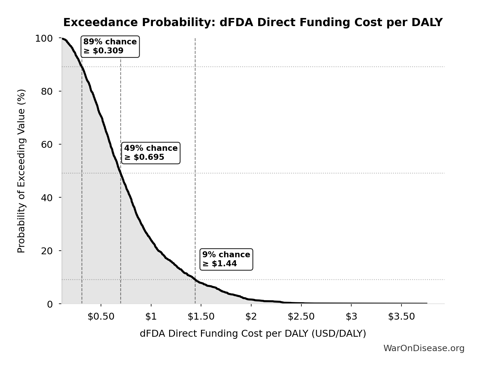
| 90% Range (5th-95th percentile) | [$0.242, $1.75] |
The histogram shows the distribution of dFDA Direct Funding Cost per DALY across 10,000 Monte Carlo simulations. The CDF (right) shows the probability of the outcome exceeding any given value, which is useful for risk assessment.
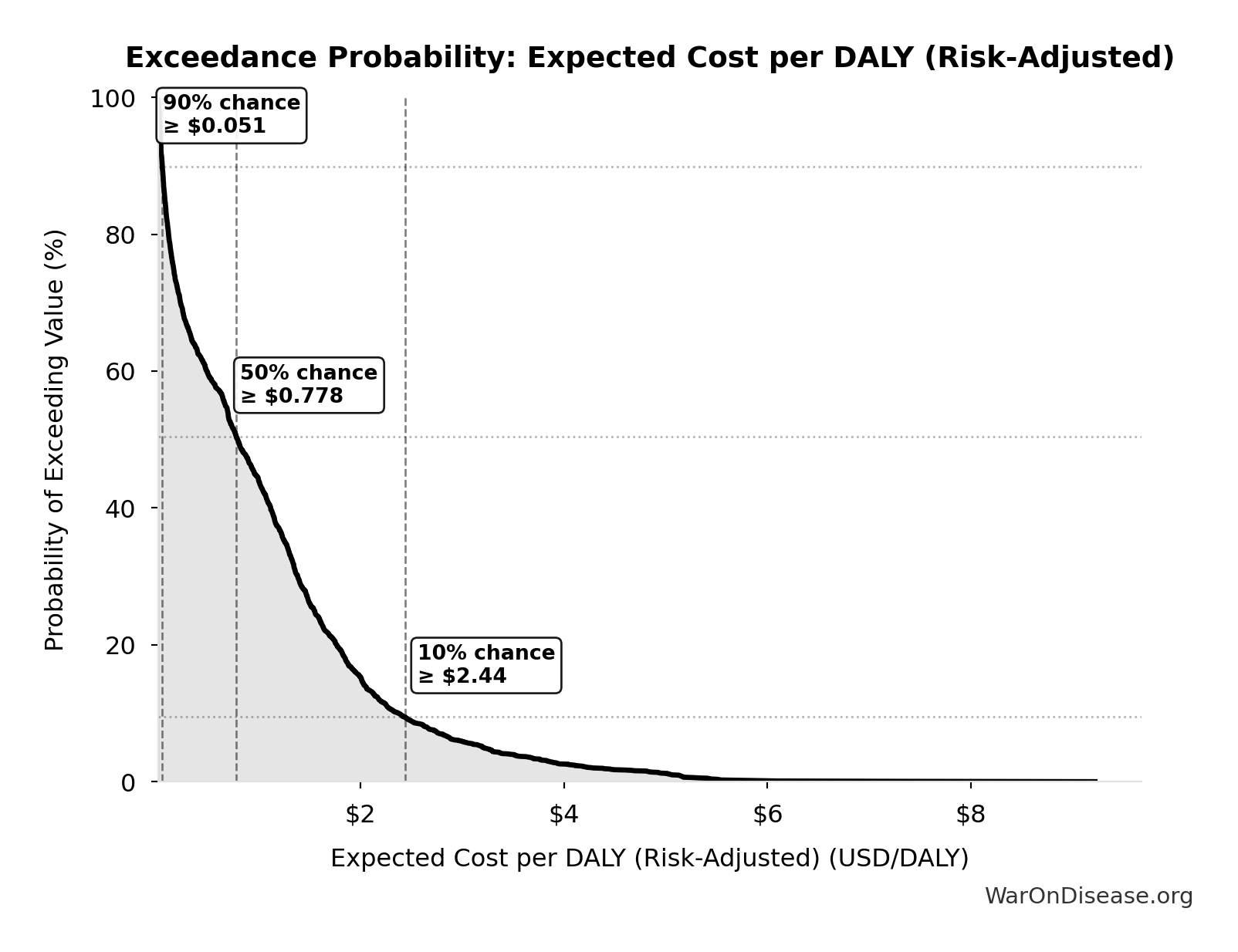
Exceedance Probability
This exceedance probability chart shows the likelihood that dFDA Direct Funding Cost per DALY will exceed any given threshold. Higher curves indicate more favorable outcomes with greater certainty.
dFDA Direct Funding NPV (Exploration Period): $476B
NPV of annual direct funding for the therapeutic space exploration period. Funding period equals exploration time (queue clearance years at given capacity multiplier). After exploration completes, the full timeline shift benefit is realized.
Inputs:
- dFDA Annual Trial Funding: $21.8B
- Standard Discount Rate for NPV Analysis: 3%
- dFDA Therapeutic Space Exploration Time 🔢: 36 years
\[ NPV_{direct} = Funding_{ann} \times \frac{1 - (1+r)^{-T}}{r} \]
✓ High confidence
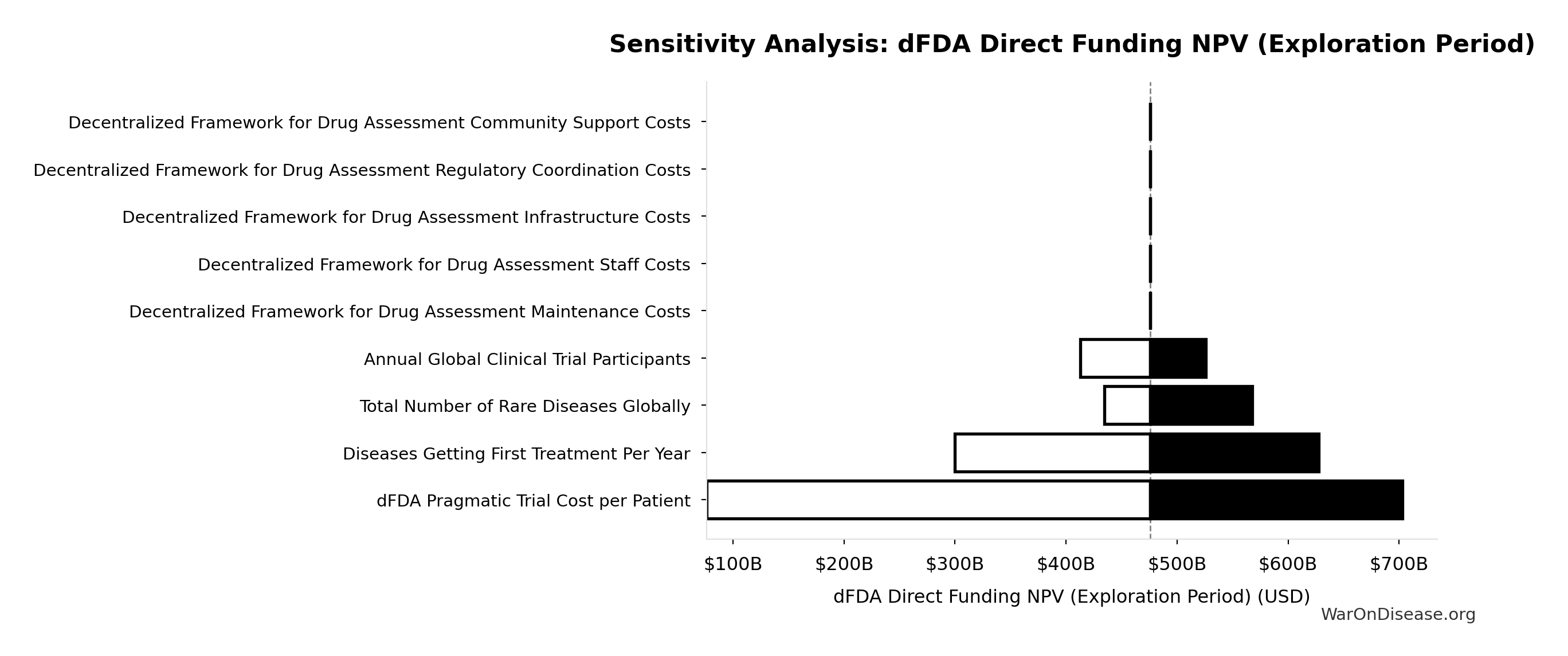
Sensitivity Analysis
Sensitivity Indices for dFDA Direct Funding NPV (Exploration Period)
Regression-based sensitivity showing which inputs explain the most variance in the output.
| Input Parameter | Sensitivity Coefficient | Interpretation |
|---|---|---|
| dFDA Therapeutic Space Exploration Time (years) | 0.9444 | Strong driver |
Interpretation: Standardized coefficients show the change in output (in SD units) per 1 SD change in input. Values near ±1 indicate strong influence; values exceeding ±1 may occur with correlated inputs.
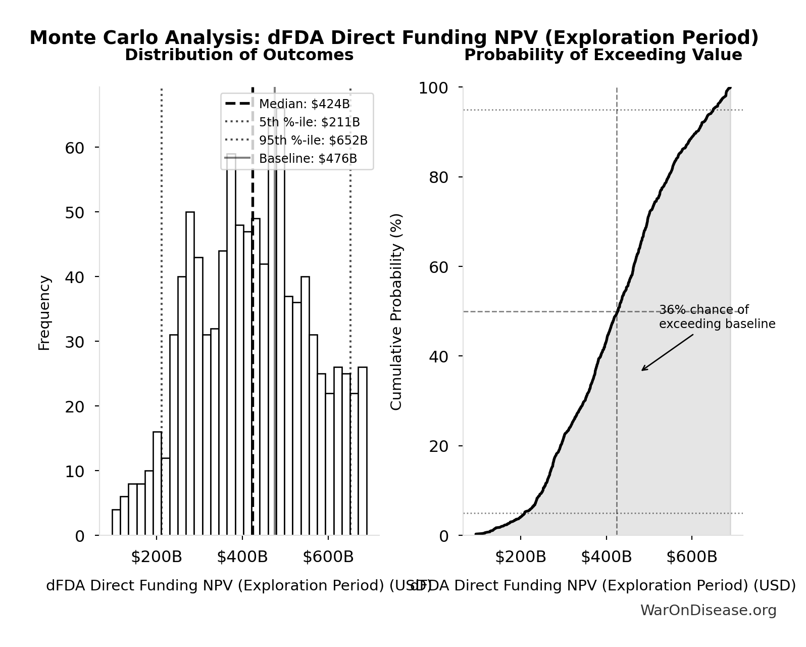
Monte Carlo Distribution
Simulation Results Summary: dFDA Direct Funding NPV (Exploration Period)
| Statistic | Value |
|---|---|
| Baseline (deterministic) | $476B |
| Mean (expected value) | $426B |
| Median (50th percentile) | $424B |
| Standard Deviation | $135B |
| 90% Range (5th-95th percentile) | [$211B, $652B] |
The histogram shows the distribution of dFDA Direct Funding NPV (Exploration Period) across 10,000 Monte Carlo simulations. The CDF (right) shows the probability of the outcome exceeding any given value, which is useful for risk assessment.
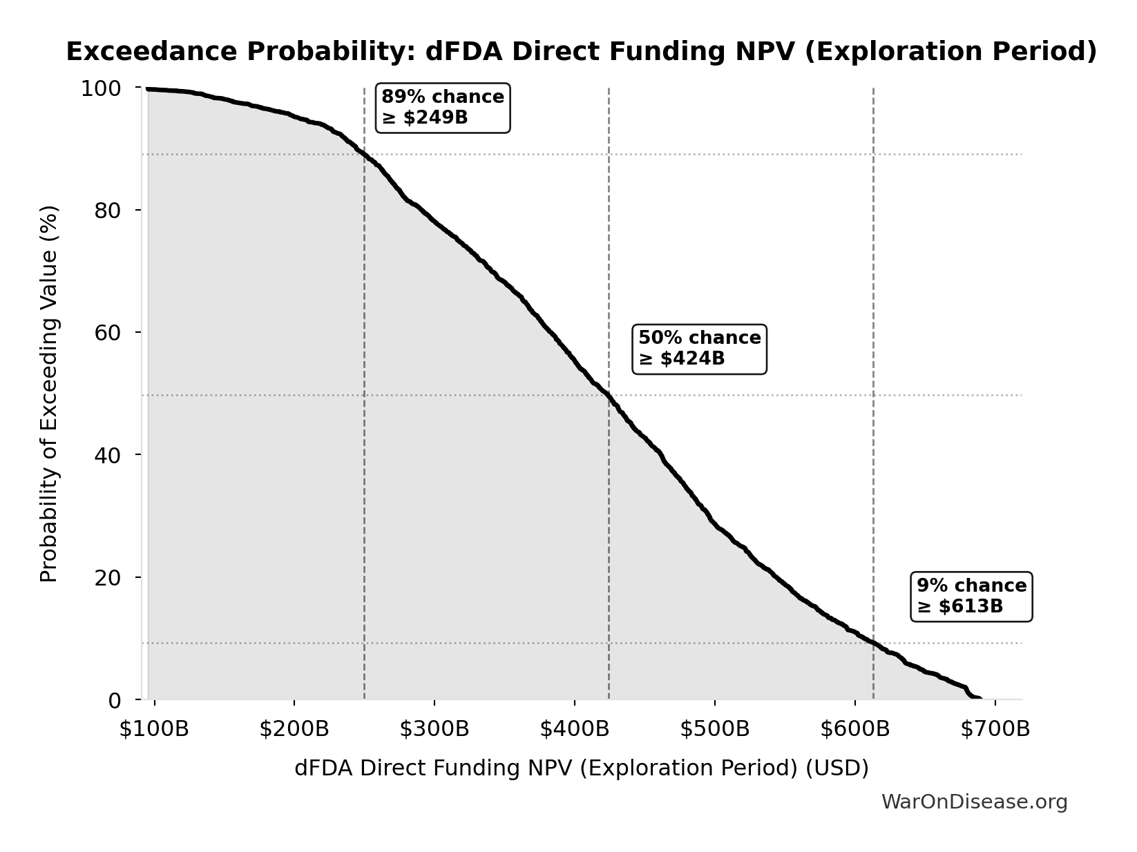
Exceedance Probability
This exceedance probability chart shows the likelihood that dFDA Direct Funding NPV (Exploration Period) will exceed any given threshold. Higher curves indicate more favorable outcomes with greater certainty.
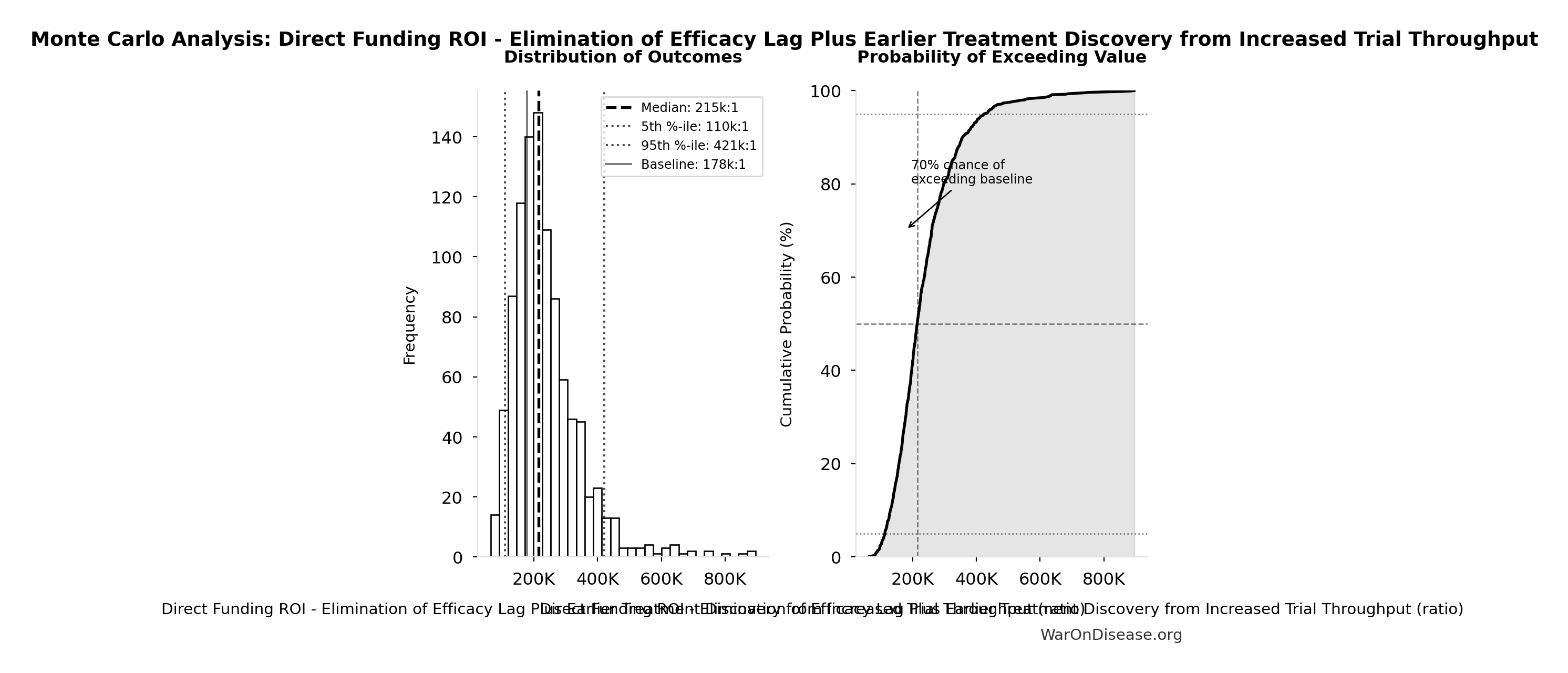
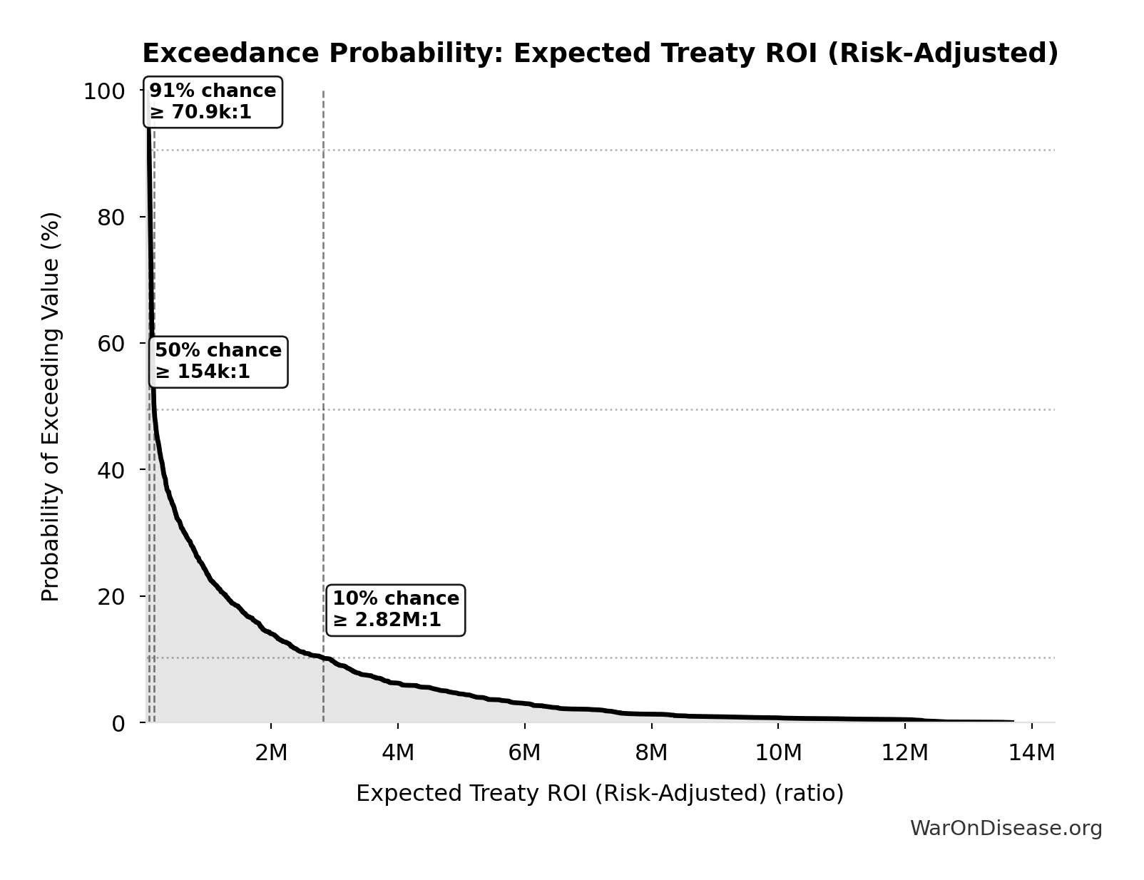
Direct Funding ROI - Elimination of Efficacy Lag Plus Earlier Treatment Discovery from Increased Trial Throughput: 178k:1
ROI from directly funding pragmatic clinical trials over the therapeutic space exploration period.
Inputs:
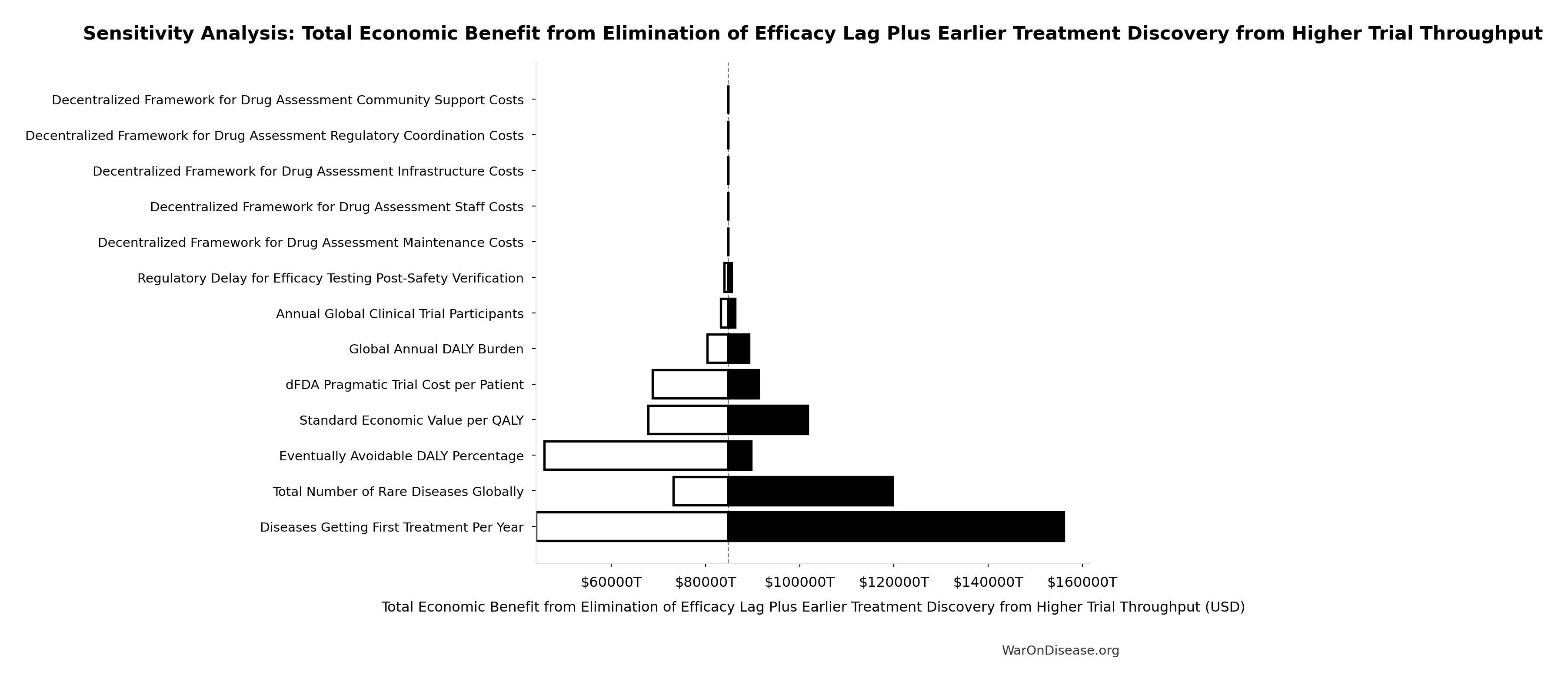
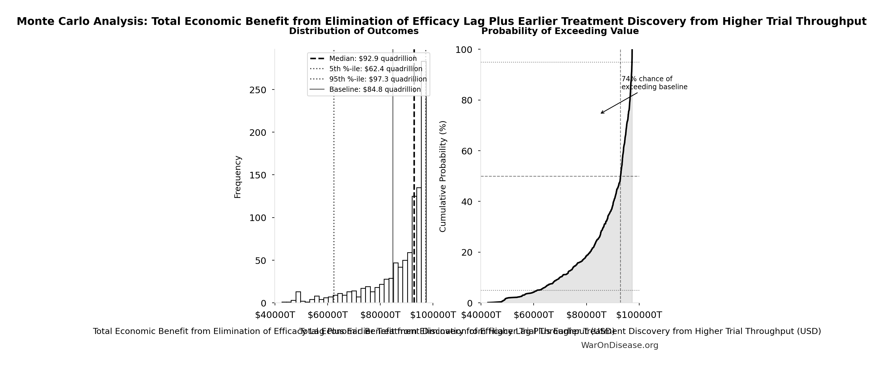
- Total Economic Benefit from Elimination of Efficacy Lag Plus Earlier Treatment Discovery from Higher Trial Throughput 🔢: $84.8 quadrillion
- dFDA Direct Funding NPV (Exploration Period) 🔢: $476B
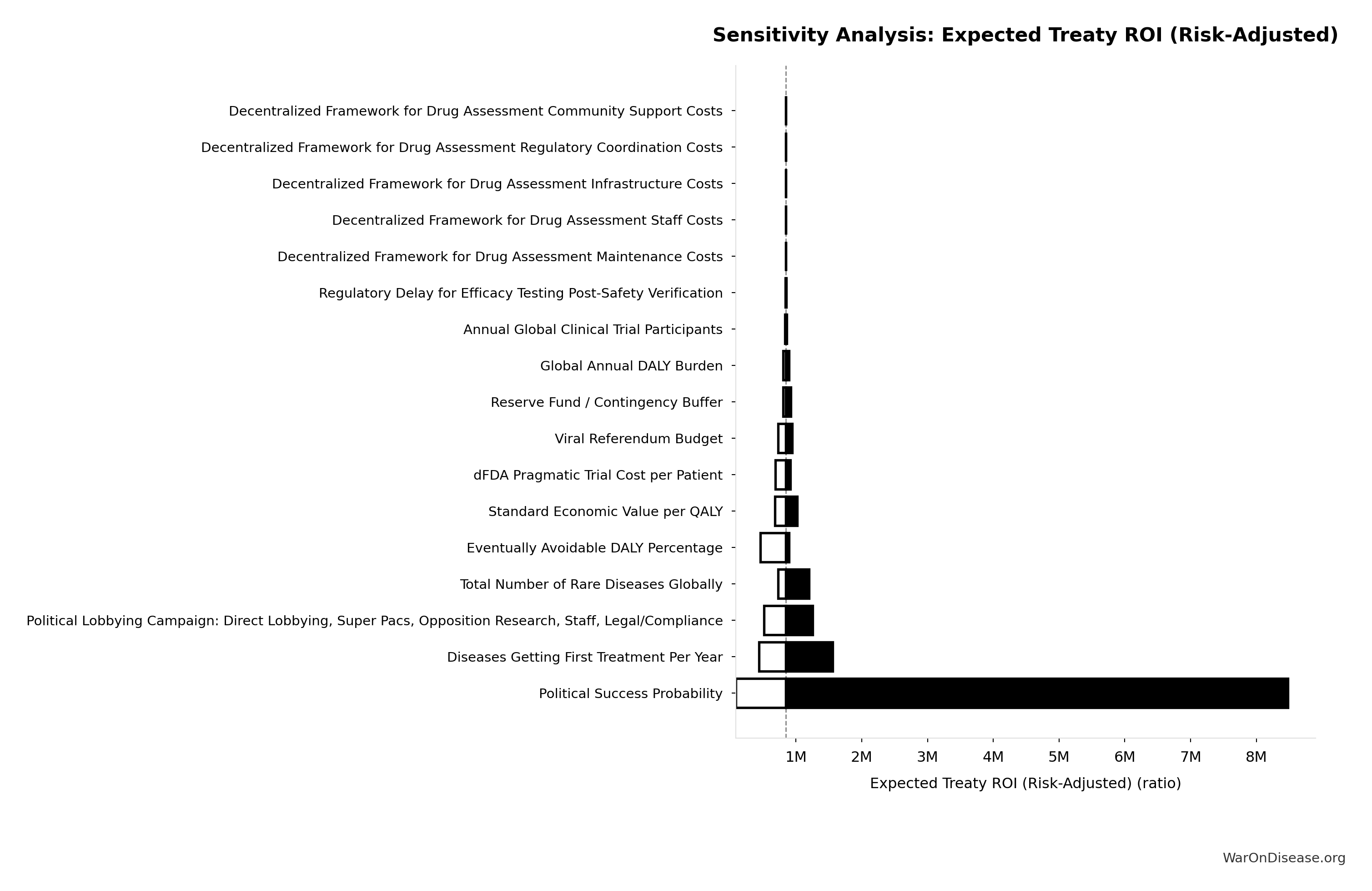
\[ \begin{gathered} ROI_{direct,max} \\ = \frac{Value_{max}}{NPV_{direct}} \\ = \frac{\$84800T}{\$476B} \\ = 178{,}000 \end{gathered} \] where: \[ \begin{gathered} Value_{max} \\ = DALYs_{max} \times Value_{QALY} \\ = 565B \times \$150K \\ = \$84800T \end{gathered} \] where: \[ \begin{gathered} DALYs_{max} \\ = DALYs_{global,ann} \times Pct_{avoid,DALY} \times T_{accel,max} \\ = 2.88B \times 92.6\% \times 212 \\ = 565B \end{gathered} \] where: \[ T_{accel,max} = T_{accel} + T_{lag} = 204 + 8.2 = 212 \] where: \[ \begin{gathered} T_{accel} \\ = T_{first,SQ} \times \left(1 - \frac{1}{k_{capacity}}\right) \\ = 222 \times \left(1 - \frac{1}{12.3}\right) \\ = 204 \end{gathered} \] where: \[ \begin{gathered} T_{first,SQ} \\ = T_{queue,SQ} \times 0.5 \\ = 443 \times 0.5 \\ = 222 \end{gathered} \] where: \[ \begin{gathered} T_{queue,SQ} \\ = \frac{N_{untreated}}{Treatments_{new,ann}} \\ = \frac{6{,}650}{15} \\ = 443 \end{gathered} \] where: \[ \begin{gathered} N_{untreated} \\ = N_{rare} \times 0.95 \\ = 7{,}000 \times 0.95 \\ = 6{,}650 \end{gathered} \] where: \[ \begin{gathered} k_{capacity} \\ = \frac{N_{fundable,dFDA}}{Slots_{curr}} \\ = \frac{23.4M}{1.9M} \\ = 12.3 \end{gathered} \] where: \[ \begin{gathered} N_{fundable,dFDA} \\ = \frac{Subsidies_{dFDA,ann}}{Cost_{pragmatic,pt}} \\ = \frac{\$21.8B}{\$929} \\ = 23.4M \end{gathered} \] where: \[ \begin{gathered} Subsidies_{dFDA,ann} \\ = Funding_{dFDA,ann} - OPEX_{dFDA} \\ = \$21.8B - \$40M \\ = \$21.8B \end{gathered} \] where: \[ \begin{gathered} OPEX_{dFDA} \\ = Cost_{platform} + Cost_{staff} + Cost_{infra} \\ + Cost_{regulatory} + Cost_{community} \\ = \$15M + \$10M + \$8M + \$5M + \$2M \\ = \$40M \end{gathered} \] where: \[ NPV_{direct} = Funding_{ann} \times \frac{1 - (1+r)^{-T}}{r} \] where: \[ \begin{gathered} T_{queue,dFDA} \\ = \frac{T_{queue,SQ}}{k_{capacity}} \\ = \frac{443}{12.3} \\ = 36 \end{gathered} \] ✓ High confidence
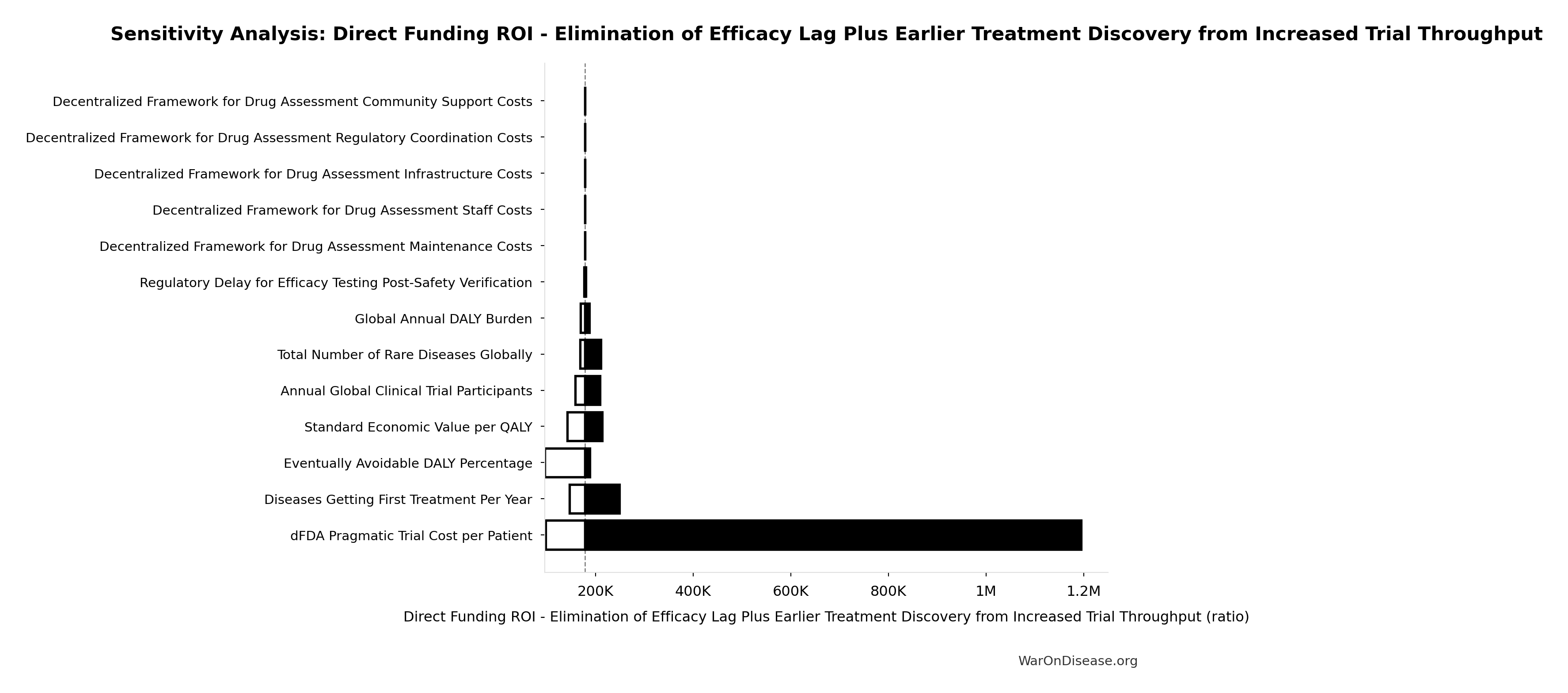
Sensitivity Analysis
Sensitivity Indices for Direct Funding ROI - Elimination of Efficacy Lag Plus Earlier Treatment Discovery from Increased Trial Throughput
Regression-based sensitivity showing which inputs explain the most variance in the output.
| Input Parameter | Sensitivity Coefficient | Interpretation |
|---|---|---|
| dFDA Direct Funding NPV (Exploration Period) (USD) | -0.8466 | Strong driver |
| Total Economic Benefit from Elimination of Efficacy Lag Plus Earlier Treatment Discovery from Higher Trial Throughput (USD) | 0.1502 | Weak driver |
Interpretation: Standardized coefficients show the change in output (in SD units) per 1 SD change in input. Values near ±1 indicate strong influence; values exceeding ±1 may occur with correlated inputs.
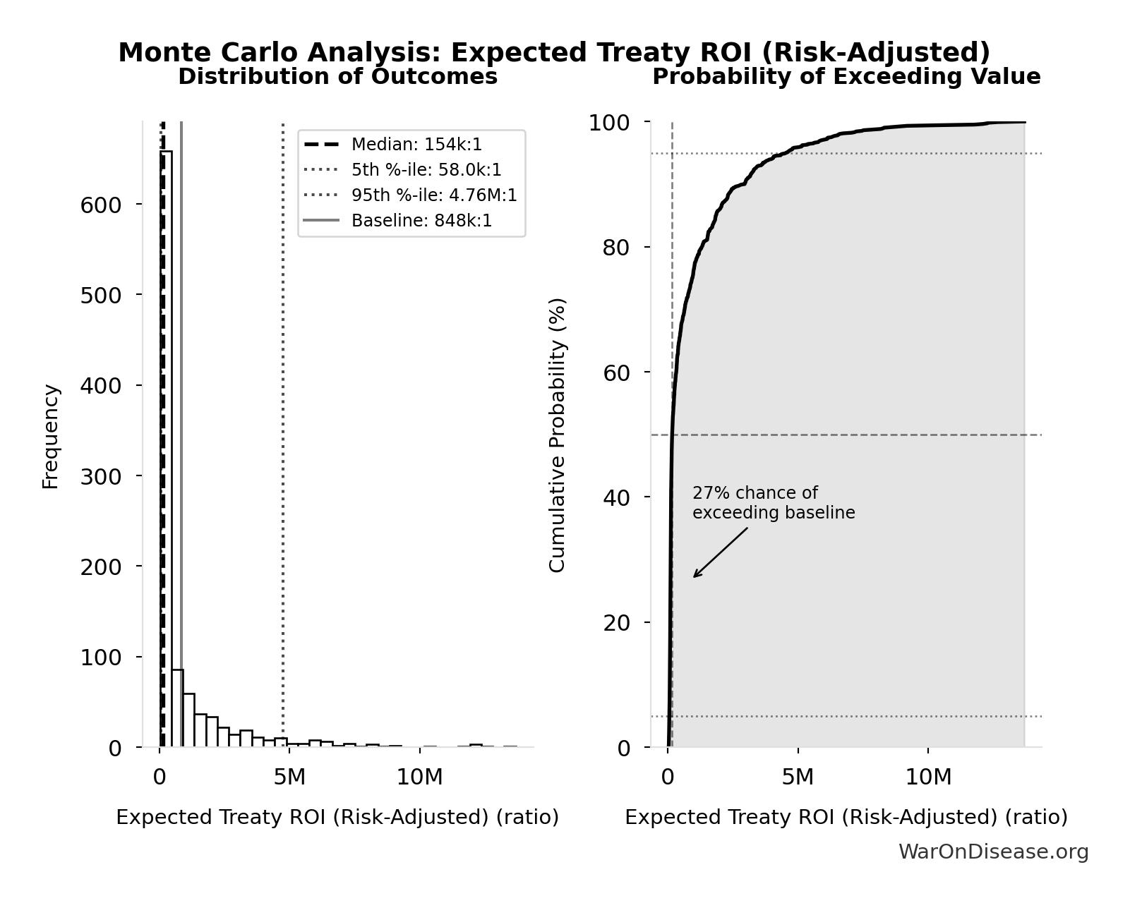
Monte Carlo Distribution
Simulation Results Summary: Direct Funding ROI - Elimination of Efficacy Lag Plus Earlier Treatment Discovery from Increased Trial Throughput
| Statistic | Value |
|---|---|
| Baseline (deterministic) | 178k:1 |
| Mean (expected value) | 236k:1 |
| Median (50th percentile) | 215k:1 |
| Standard Deviation | 106k:1 |
| 90% Range (5th-95th percentile) | [110k:1, 421k:1] |
The histogram shows the distribution of Direct Funding ROI - Elimination of Efficacy Lag Plus Earlier Treatment Discovery from Increased Trial Throughput across 10,000 Monte Carlo simulations. The CDF (right) shows the probability of the outcome exceeding any given value, which is useful for risk assessment.
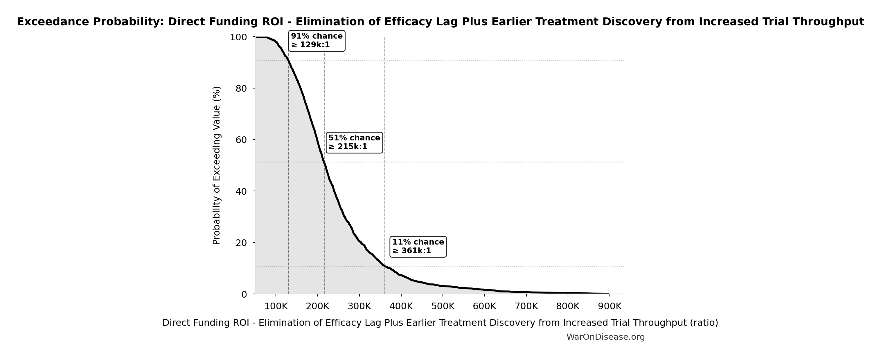
Exceedance Probability
This exceedance probability chart shows the likelihood that Direct Funding ROI - Elimination of Efficacy Lag Plus Earlier Treatment Discovery from Increased Trial Throughput will exceed any given threshold. Higher curves indicate more favorable outcomes with greater certainty.
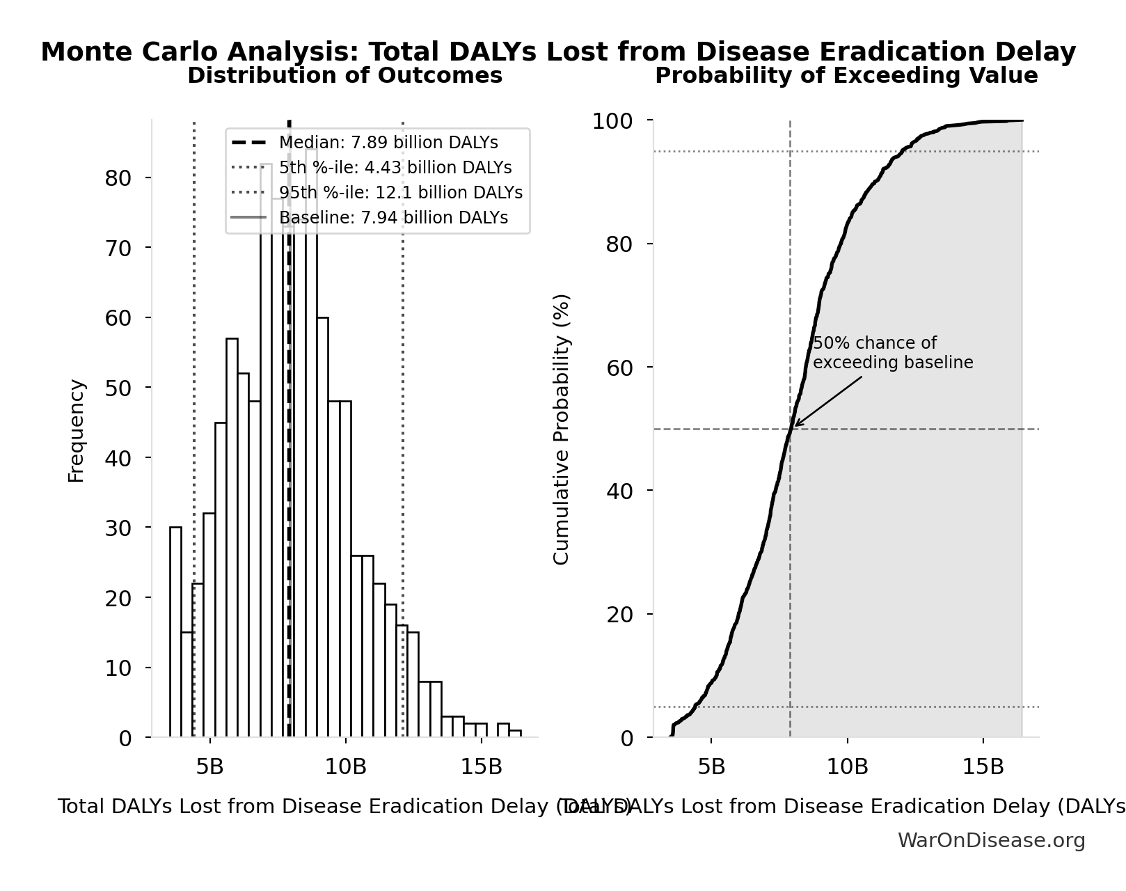
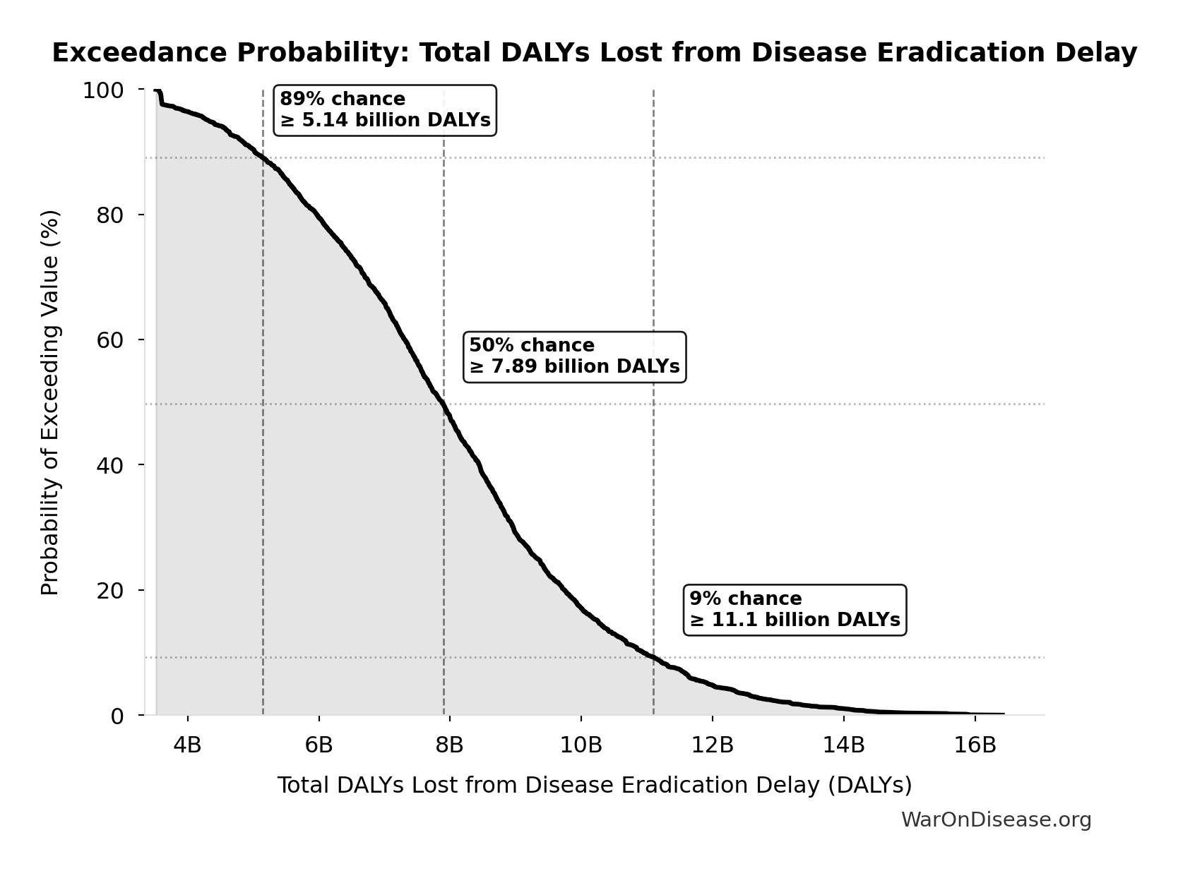
Total DALYs Lost from Disease Eradication Delay: 7.94 billion DALYs
Total Disability-Adjusted Life Years lost from disease eradication delay (PRIMARY estimate)
Inputs:
- Years of Life Lost from Disease Eradication Delay 🔢: 7.07 billion years
- Years Lived with Disability During Disease Eradication Delay 🔢: 873 million years
\[ DALYs_{lag} = YLL_{lag} + YLD_{lag} = 7.07B + 873M = 7.94B \] where: \[ \begin{gathered} YLL_{lag} \\ = Deaths_{lag} \times (LE_{global} - Age_{death,delay}) \\ = 416M \times (79 - 62) \\ = 7.07B \end{gathered} \] where: \[ \begin{gathered} Deaths_{lag} \\ = T_{lag} \times Deaths_{disease,daily} \times 338 \\ = 8.2 \times 150{,}000 \times 338 \\ = 416M \end{gathered} \] where: \[ \begin{gathered} YLD_{lag} \\ = Deaths_{lag} \times T_{suffering} \times DW_{chronic} \\ = 416M \times 6 \times 0.35 \\ = 873M \end{gathered} \] ~ Medium confidence
Sensitivity Analysis
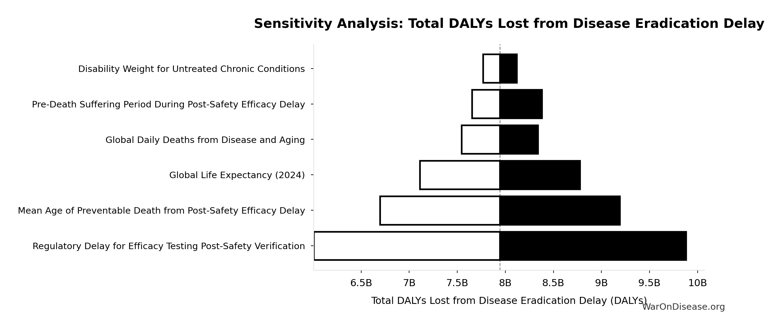
Sensitivity Indices for Total DALYs Lost from Disease Eradication Delay
Regression-based sensitivity showing which inputs explain the most variance in the output.
| Input Parameter | Sensitivity Coefficient | Interpretation |
|---|---|---|
| Years of Life Lost from Disease Eradication Delay (years) | 0.7043 | Strong driver |
| Years Lived with Disability During Disease Eradication Delay (years) | 0.3107 | Moderate driver |
Interpretation: Standardized coefficients show the change in output (in SD units) per 1 SD change in input. Values near ±1 indicate strong influence; values exceeding ±1 may occur with correlated inputs.
Monte Carlo Distribution
Simulation Results Summary: Total DALYs Lost from Disease Eradication Delay
| Statistic | Value |
|---|---|
| Baseline (deterministic) | 7.94 billion |
| Mean (expected value) | 8.05 billion |
| Median (50th percentile) | 7.89 billion |
| Standard Deviation | 2.31 billion |
| 90% Range (5th-95th percentile) | [4.43 billion, 12.1 billion] |
The histogram shows the distribution of Total DALYs Lost from Disease Eradication Delay across 10,000 Monte Carlo simulations. The CDF (right) shows the probability of the outcome exceeding any given value, which is useful for risk assessment.
Exceedance Probability
This exceedance probability chart shows the likelihood that Total DALYs Lost from Disease Eradication Delay will exceed any given threshold. Higher curves indicate more favorable outcomes with greater certainty.
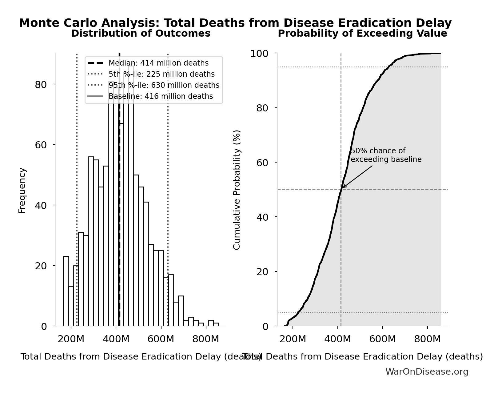
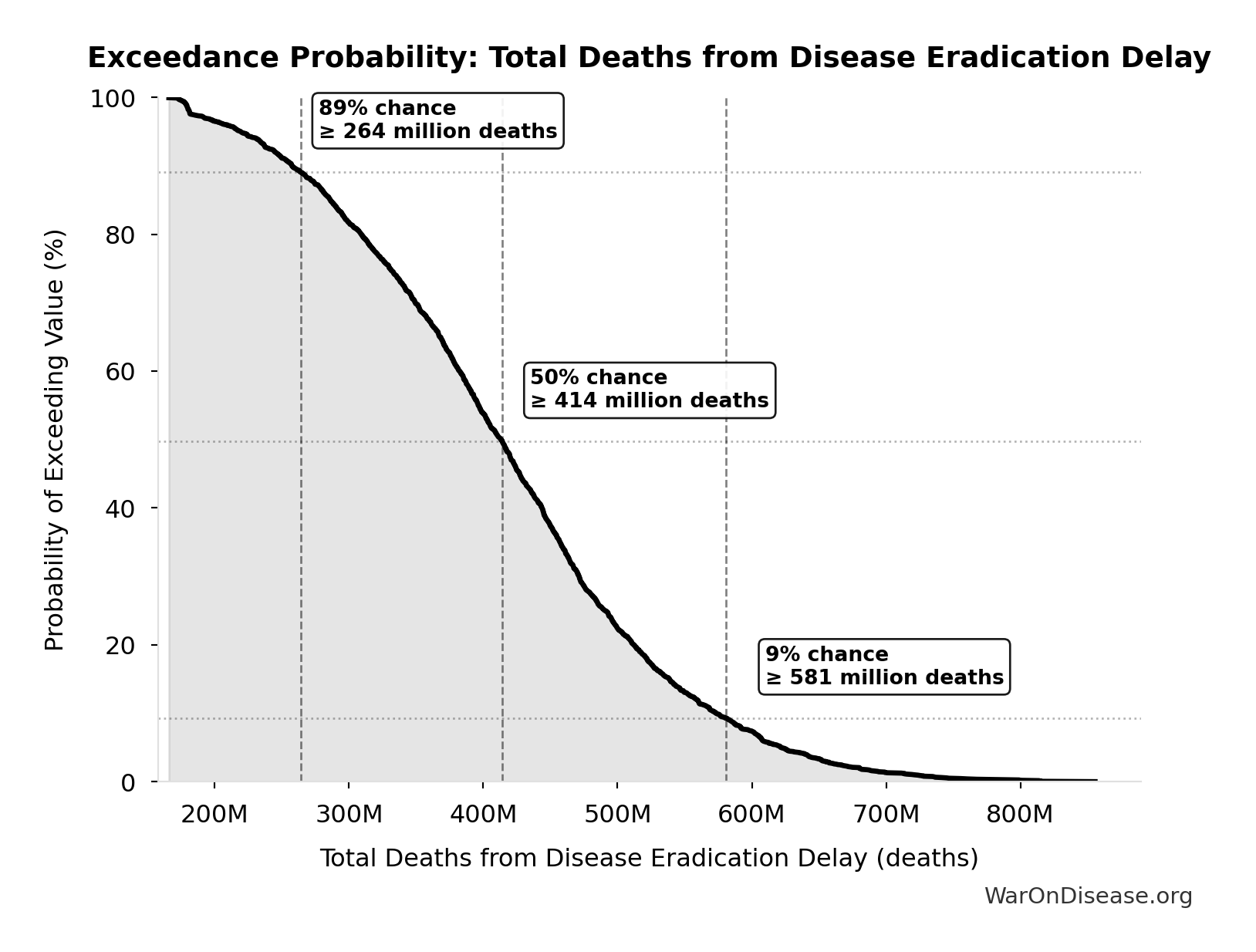
Total Deaths from Disease Eradication Delay: 416 million deaths
Total eventually avoidable deaths from delaying disease eradication by 8.2 years (PRIMARY estimate, conservative). Excludes fundamentally unavoidable deaths (primarily accidents ~7.9%).
Inputs:
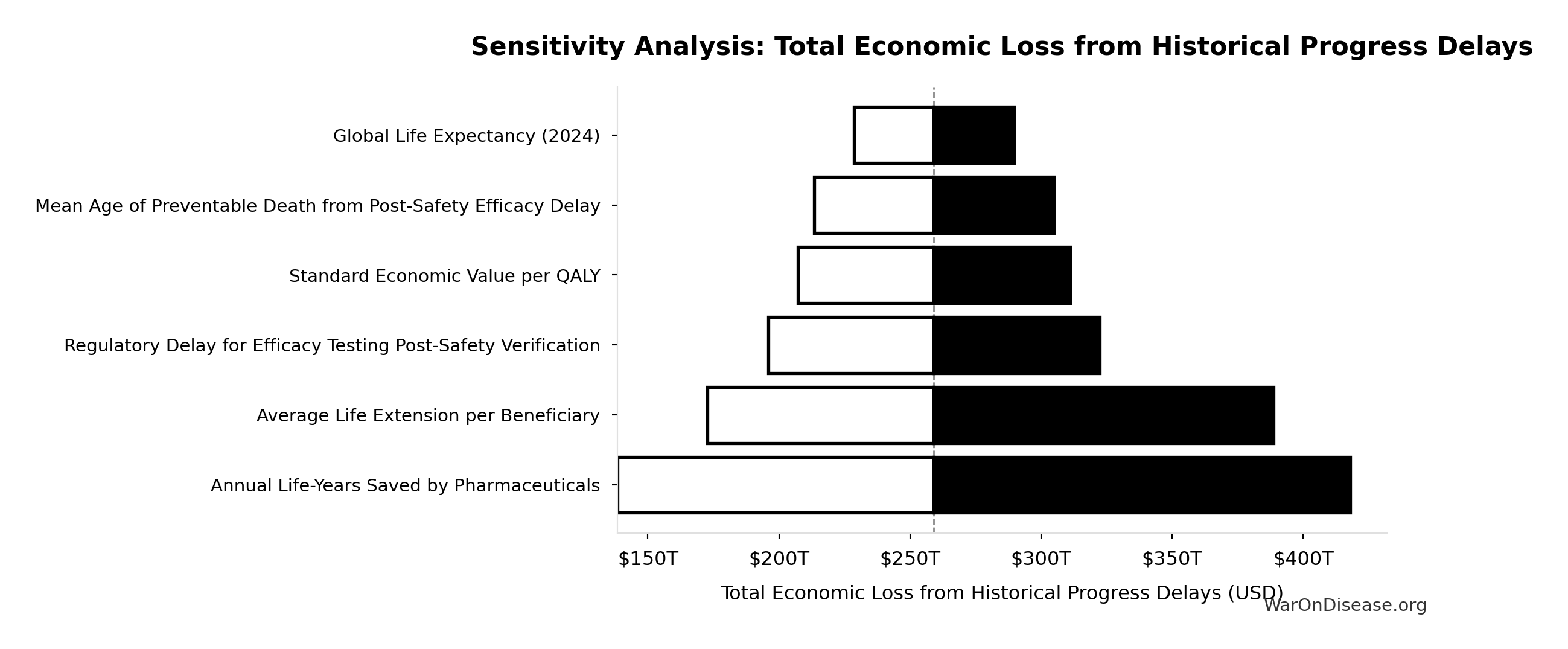
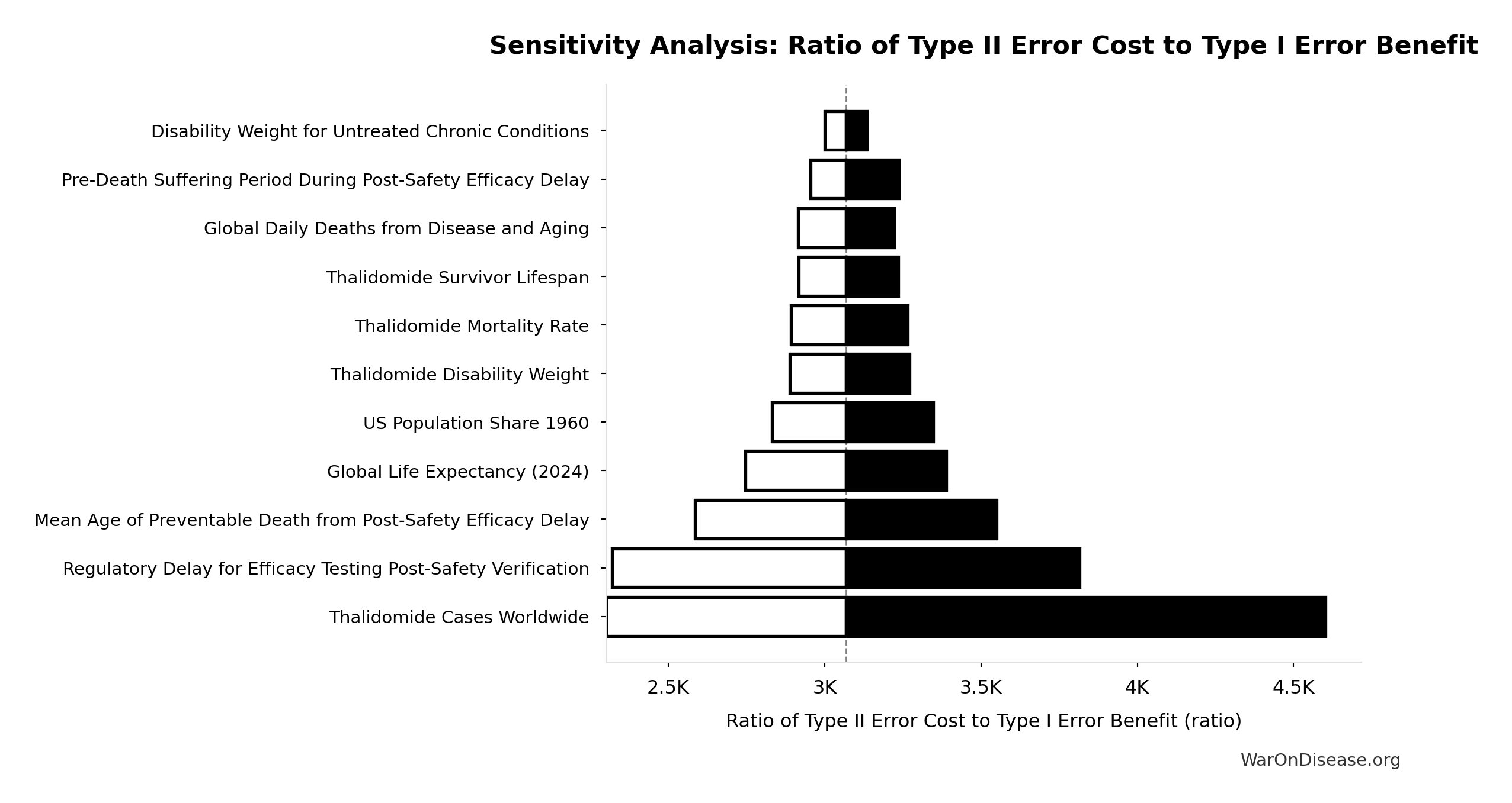
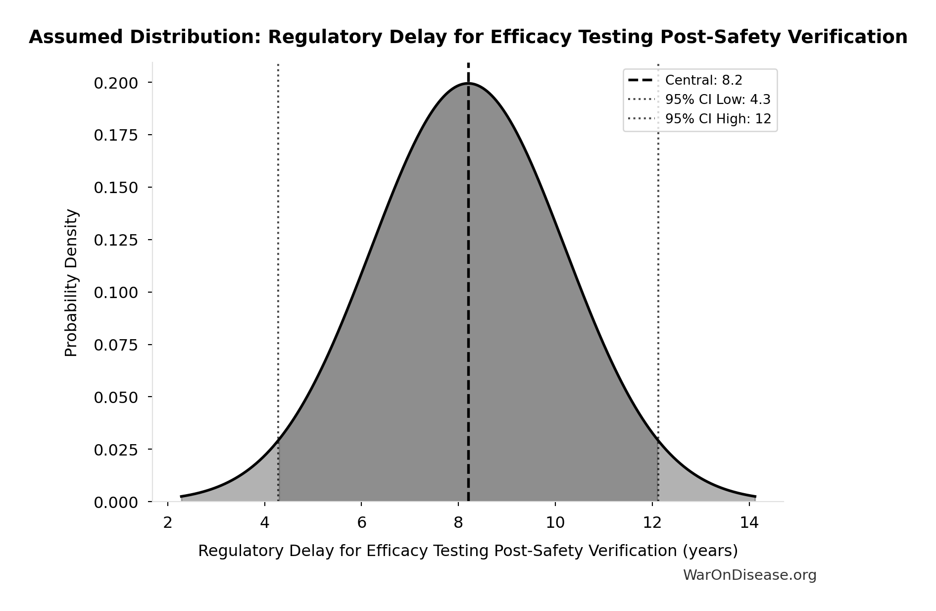
- Regulatory Delay for Efficacy Testing Post-Safety Verification 📊: 8.2 years (SE: ±2 years)
- Global Daily Deaths from Disease and Aging 📊: 150 thousand deaths/day (SE: ±7.5 thousand deaths/day)
\[ \begin{gathered} Deaths_{lag} \\ = T_{lag} \times Deaths_{disease,daily} \times 338 \\ = 8.2 \times 150{,}000 \times 338 \\ = 416M \end{gathered} \]
~ Medium confidence
Sensitivity Analysis
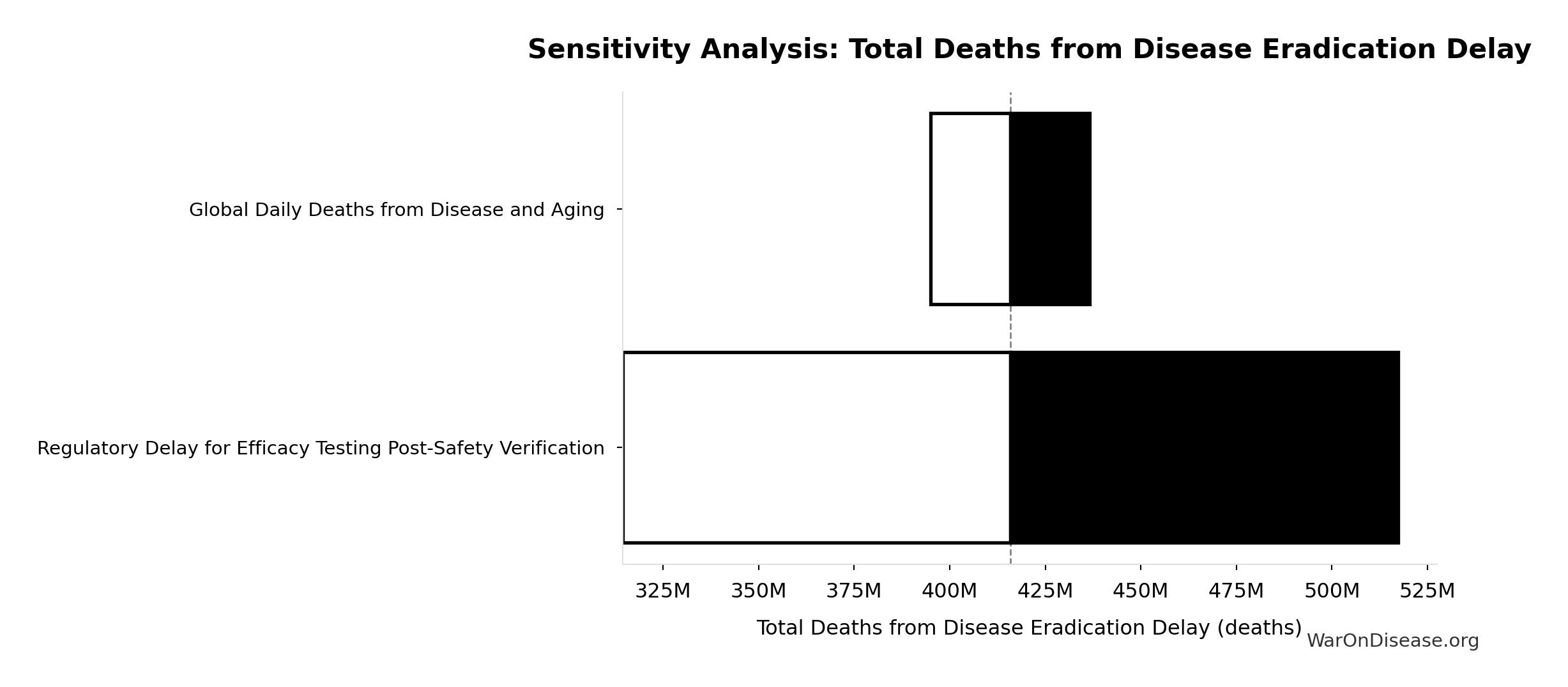
Sensitivity Indices for Total Deaths from Disease Eradication Delay
Regression-based sensitivity showing which inputs explain the most variance in the output.
| Input Parameter | Sensitivity Coefficient | Interpretation |
|---|---|---|
| Regulatory Delay for Efficacy Testing Post-Safety Verification (years) | 1.1404 | Strong driver |
| Global Daily Deaths from Disease and Aging (deaths/day) | -0.1422 | Weak driver |
Interpretation: Standardized coefficients show the change in output (in SD units) per 1 SD change in input. Values near ±1 indicate strong influence; values exceeding ±1 may occur with correlated inputs.
Monte Carlo Distribution
Simulation Results Summary: Total Deaths from Disease Eradication Delay
| Statistic | Value |
|---|---|
| Baseline (deterministic) | 416 million |
| Mean (expected value) | 420 million |
| Median (50th percentile) | 414 million |
| Standard Deviation | 122 million |
| 90% Range (5th-95th percentile) | [225 million, 630 million] |
The histogram shows the distribution of Total Deaths from Disease Eradication Delay across 10,000 Monte Carlo simulations. The CDF (right) shows the probability of the outcome exceeding any given value, which is useful for risk assessment.
Exceedance Probability
This exceedance probability chart shows the likelihood that Total Deaths from Disease Eradication Delay will exceed any given threshold. Higher curves indicate more favorable outcomes with greater certainty.
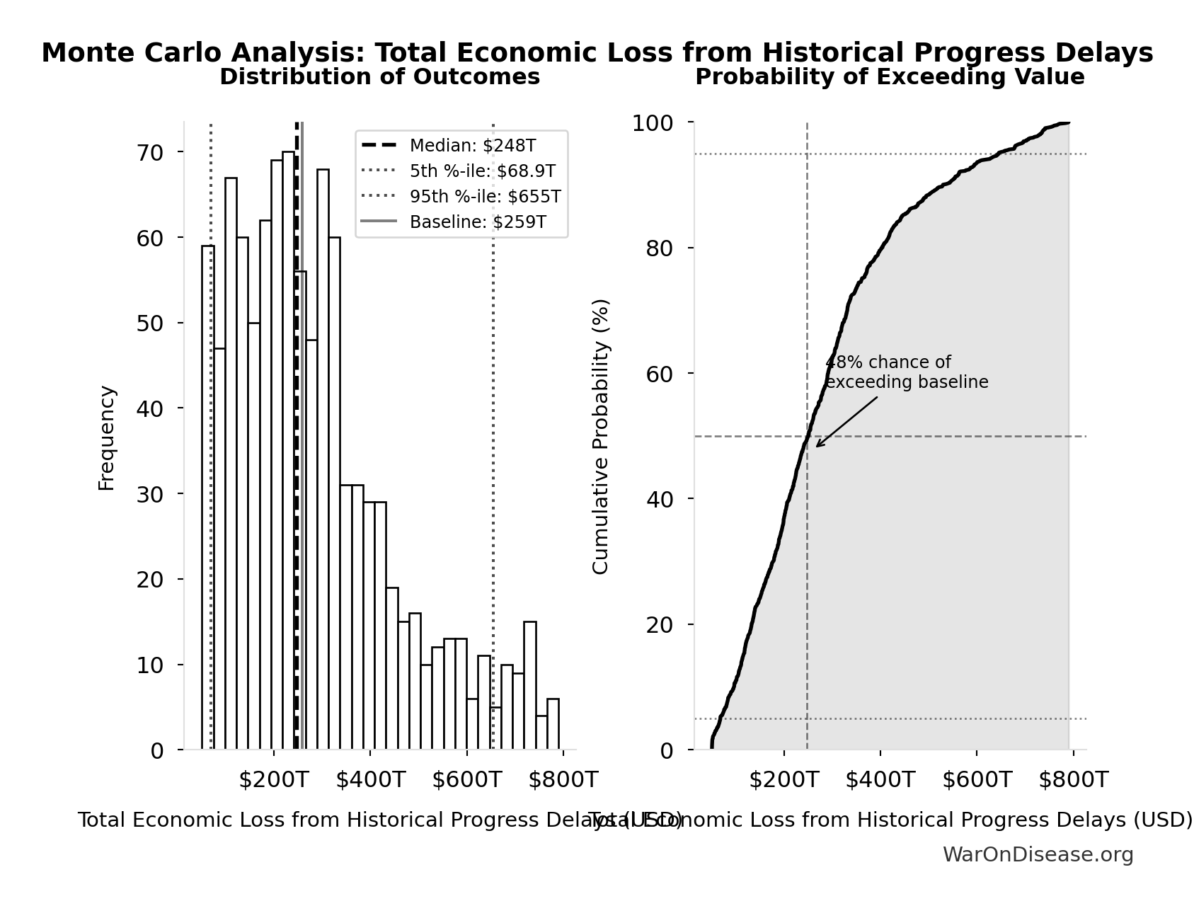
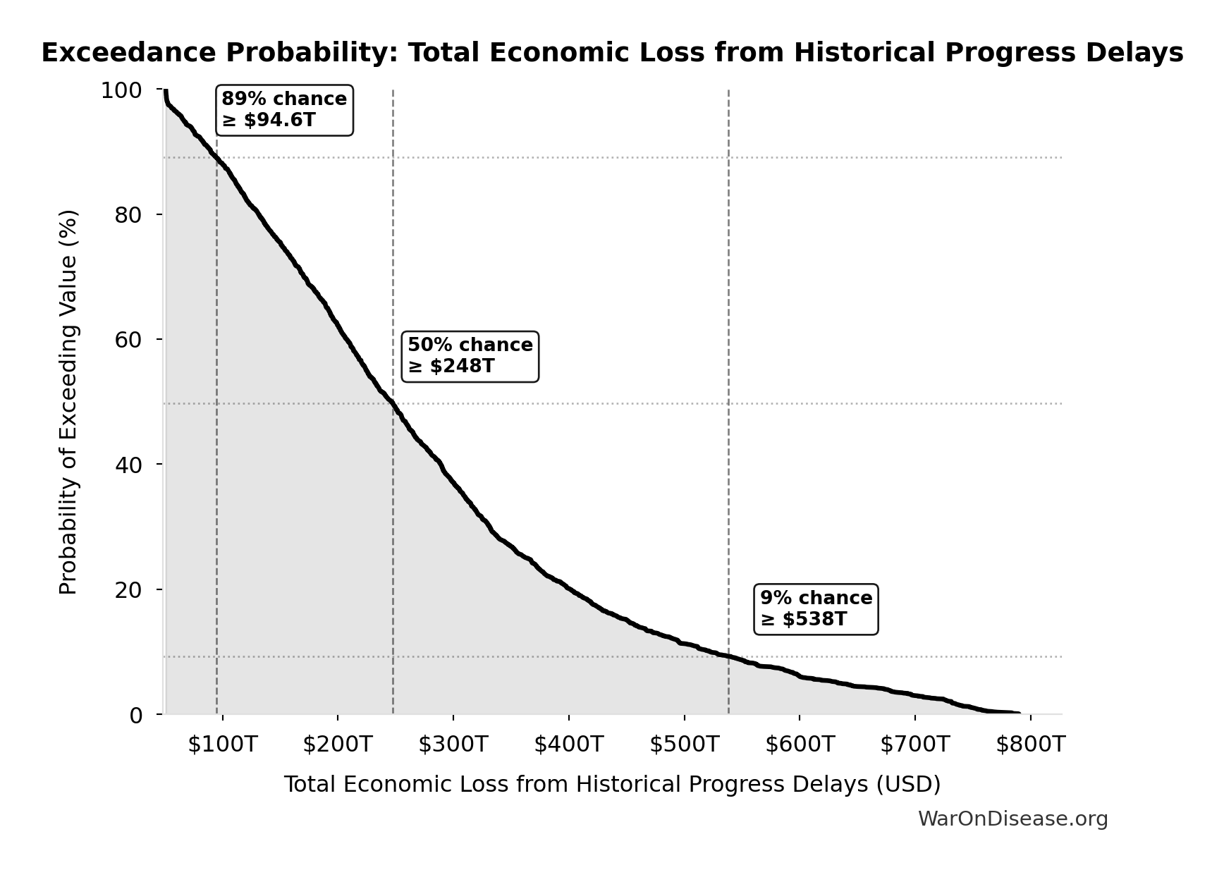
Total Economic Loss from Disease Eradication Delay: $1.19 quadrillion
Total economic loss from delaying disease eradication by 8.2 years (PRIMARY estimate, 2024 USD). Values global DALYs at standardized US/International normative rate ($150k) rather than local ability-to-pay, representing the full human capital loss.
Inputs:
- Total DALYs Lost from Disease Eradication Delay 🔢: 7.94 billion DALYs
- Standard Economic Value per QALY 📊: $150K (SE: ±$30K)
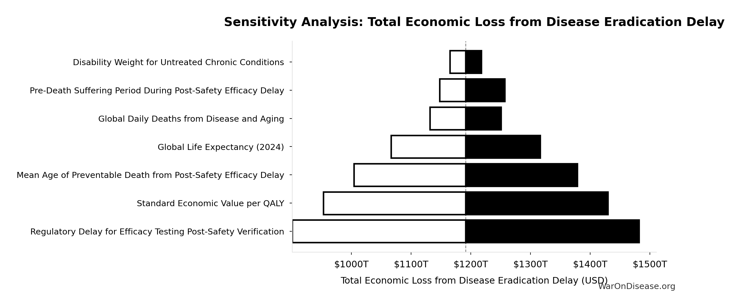
\[ \begin{gathered} Value_{lag} \\ = DALYs_{lag} \times Value_{QALY} \\ = 7.94B \times \$150K \\ = \$1190T \end{gathered} \] where: \[ DALYs_{lag} = YLL_{lag} + YLD_{lag} = 7.07B + 873M = 7.94B \] where: \[ \begin{gathered} YLL_{lag} \\ = Deaths_{lag} \times (LE_{global} - Age_{death,delay}) \\ = 416M \times (79 - 62) \\ = 7.07B \end{gathered} \] where: \[ \begin{gathered} Deaths_{lag} \\ = T_{lag} \times Deaths_{disease,daily} \times 338 \\ = 8.2 \times 150{,}000 \times 338 \\ = 416M \end{gathered} \] where: \[ \begin{gathered} YLD_{lag} \\ = Deaths_{lag} \times T_{suffering} \times DW_{chronic} \\ = 416M \times 6 \times 0.35 \\ = 873M \end{gathered} \] ~ Medium confidence
Sensitivity Analysis
Sensitivity Indices for Total Economic Loss from Disease Eradication Delay
Regression-based sensitivity showing which inputs explain the most variance in the output.
| Input Parameter | Sensitivity Coefficient | Interpretation |
|---|---|---|
| Total DALYs Lost from Disease Eradication Delay (DALYs) | 1.0671 | Strong driver |
| Standard Economic Value per QALY (USD/QALY) | -0.0733 | Minimal effect |
Interpretation: Standardized coefficients show the change in output (in SD units) per 1 SD change in input. Values near ±1 indicate strong influence; values exceeding ±1 may occur with correlated inputs.
Monte Carlo Distribution
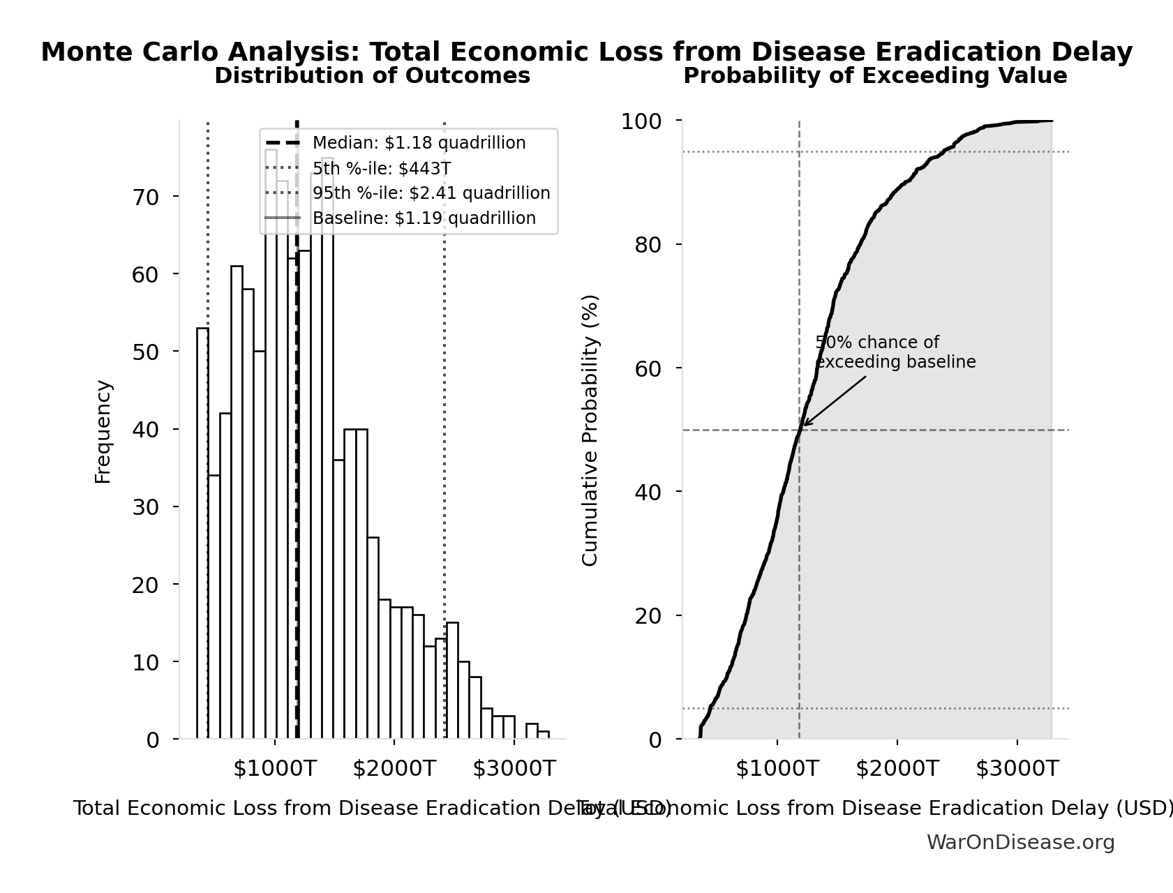
Simulation Results Summary: Total Economic Loss from Disease Eradication Delay
| Statistic | Value |
|---|---|
| Baseline (deterministic) | $1.19 quadrillion |
| Mean (expected value) | $1.27 quadrillion |
| Median (50th percentile) | $1.18 quadrillion |
| Standard Deviation | $581T |
| 90% Range (5th-95th percentile) | [$443T, $2.41 quadrillion] |
The histogram shows the distribution of Total Economic Loss from Disease Eradication Delay across 10,000 Monte Carlo simulations. The CDF (right) shows the probability of the outcome exceeding any given value, which is useful for risk assessment.
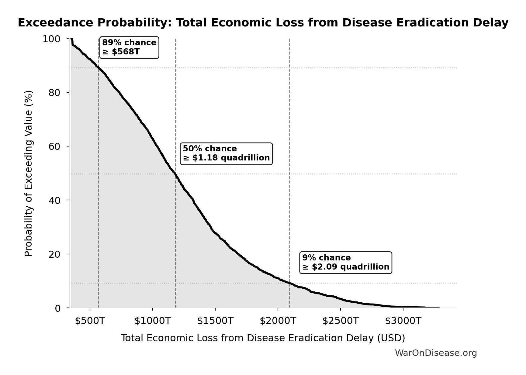
Exceedance Probability
This exceedance probability chart shows the likelihood that Total Economic Loss from Disease Eradication Delay will exceed any given threshold. Higher curves indicate more favorable outcomes with greater certainty.
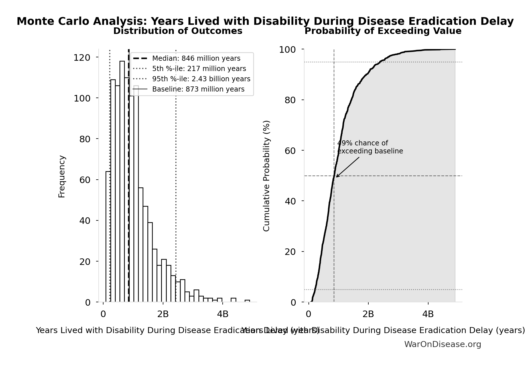
Years Lived with Disability During Disease Eradication Delay: 873 million years
Years Lived with Disability during disease eradication delay (PRIMARY estimate)
Inputs:
- Total Deaths from Disease Eradication Delay 🔢: 416 million deaths
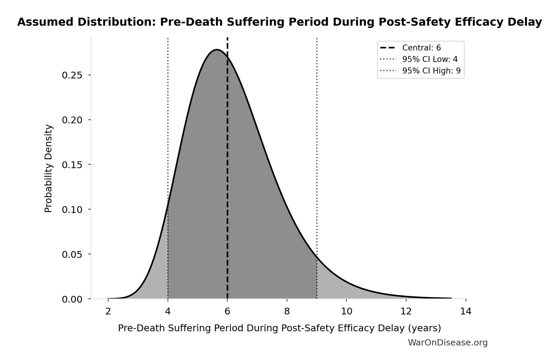
- Pre-Death Suffering Period During Post-Safety Efficacy Delay 📊: 6 years (95% CI: 4 years - 9 years)
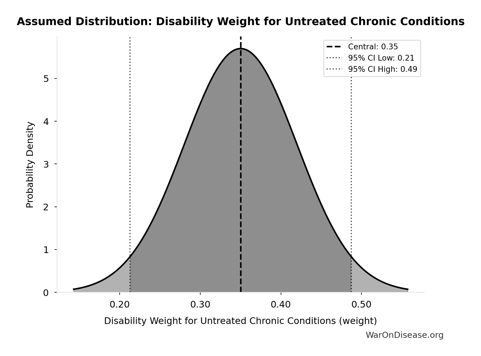
- Disability Weight for Untreated Chronic Conditions 📊: 0.35 weight (SE: ±0.07 weight)
\[ \begin{gathered} YLD_{lag} \\ = Deaths_{lag} \times T_{suffering} \times DW_{chronic} \\ = 416M \times 6 \times 0.35 \\ = 873M \end{gathered} \] where: \[ \begin{gathered} Deaths_{lag} \\ = T_{lag} \times Deaths_{disease,daily} \times 338 \\ = 8.2 \times 150{,}000 \times 338 \\ = 416M \end{gathered} \] ~ Medium confidence
Sensitivity Analysis
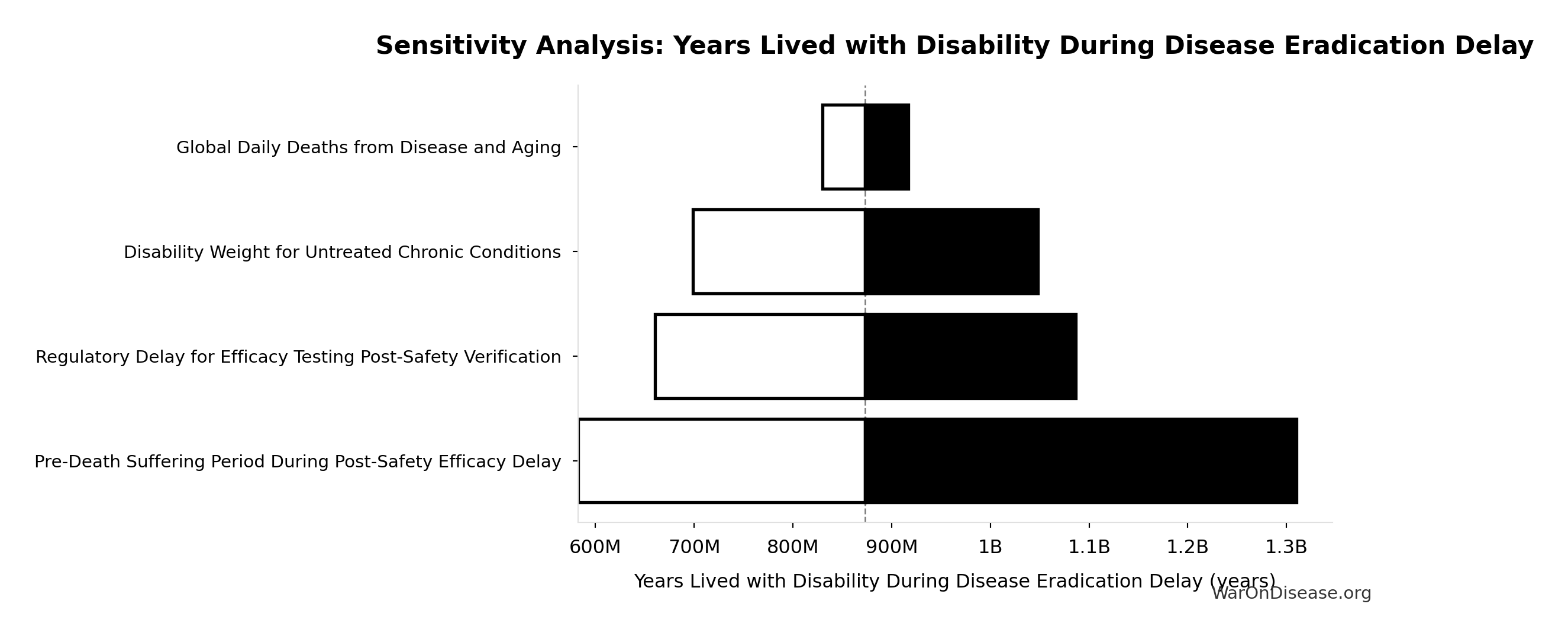
Sensitivity Indices for Years Lived with Disability During Disease Eradication Delay
Regression-based sensitivity showing which inputs explain the most variance in the output.
| Input Parameter | Sensitivity Coefficient | Interpretation |
|---|---|---|
| Pre-Death Suffering Period During Post-Safety Efficacy Delay (years) | 2.0883 | Strong driver |
| Disability Weight for Untreated Chronic Conditions (weight) | -0.9003 | Strong driver |
| Total Deaths from Disease Eradication Delay (deaths) | -0.2255 | Weak driver |
Interpretation: Standardized coefficients show the change in output (in SD units) per 1 SD change in input. Values near ±1 indicate strong influence; values exceeding ±1 may occur with correlated inputs.
Monte Carlo Distribution
Simulation Results Summary: Years Lived with Disability During Disease Eradication Delay
| Statistic | Value |
|---|---|
| Baseline (deterministic) | 873 million |
| Mean (expected value) | 1.02 billion |
| Median (50th percentile) | 846 million |
| Standard Deviation | 716 million |
| 90% Range (5th-95th percentile) | [217 million, 2.43 billion] |
The histogram shows the distribution of Years Lived with Disability During Disease Eradication Delay across 10,000 Monte Carlo simulations. The CDF (right) shows the probability of the outcome exceeding any given value, which is useful for risk assessment.
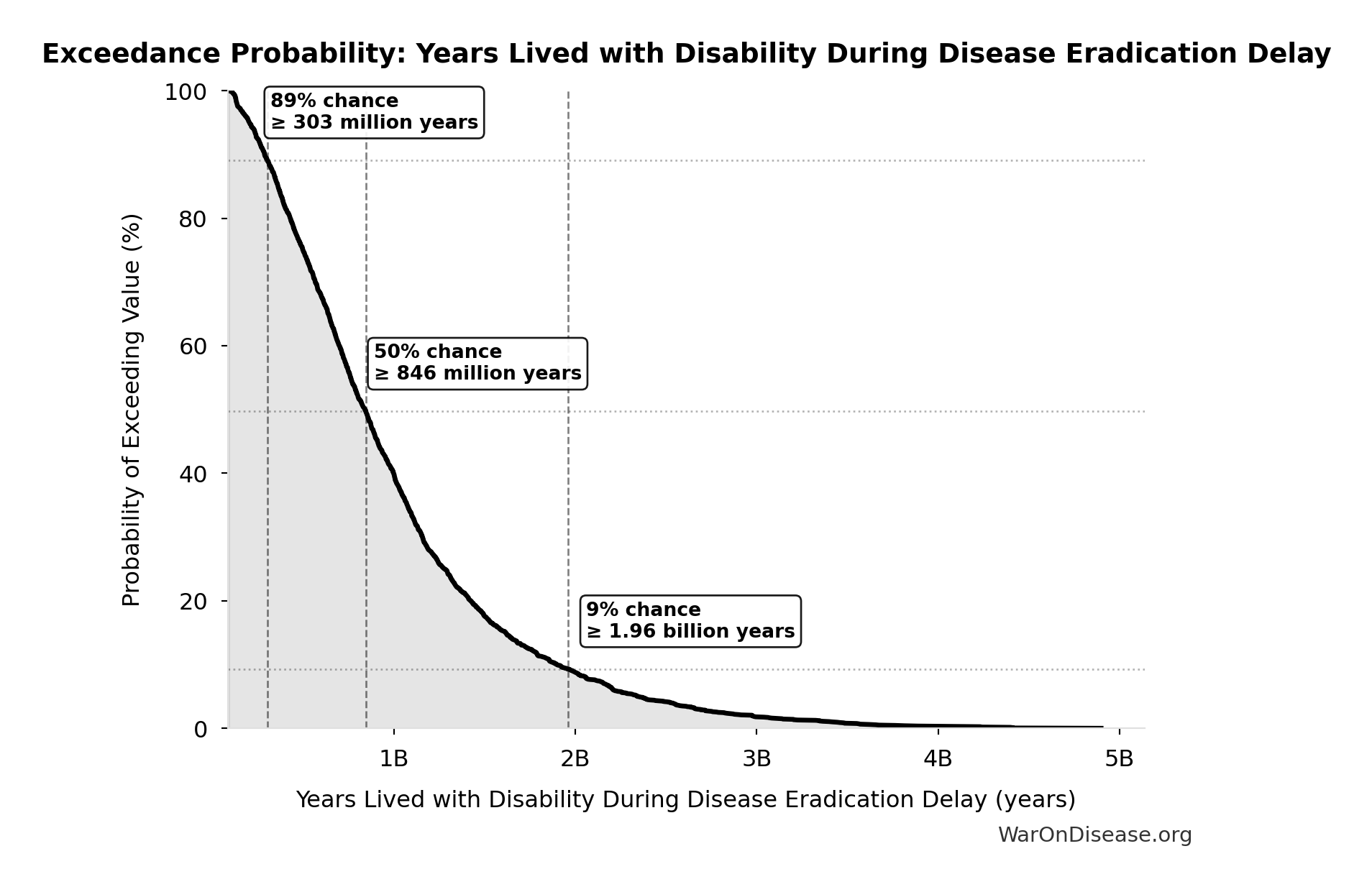
Exceedance Probability
This exceedance probability chart shows the likelihood that Years Lived with Disability During Disease Eradication Delay will exceed any given threshold. Higher curves indicate more favorable outcomes with greater certainty.
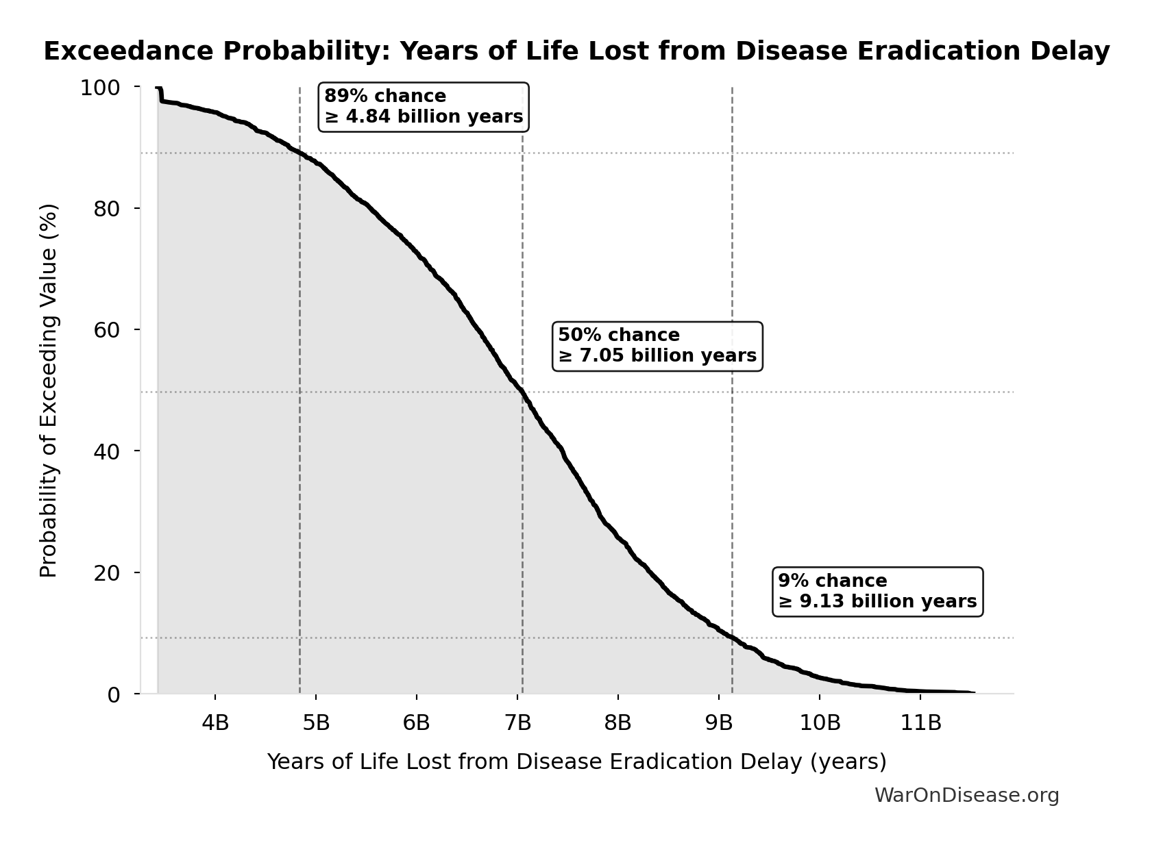
Years of Life Lost from Disease Eradication Delay: 7.07 billion years
Years of Life Lost from disease eradication delay deaths (PRIMARY estimate)
Inputs:
- Total Deaths from Disease Eradication Delay 🔢: 416 million deaths
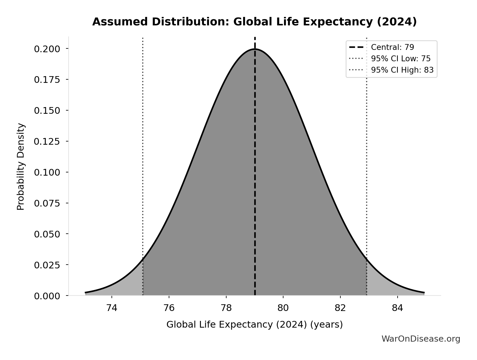
- Global Life Expectancy (2024) 📊: 79 years (SE: ±2 years)
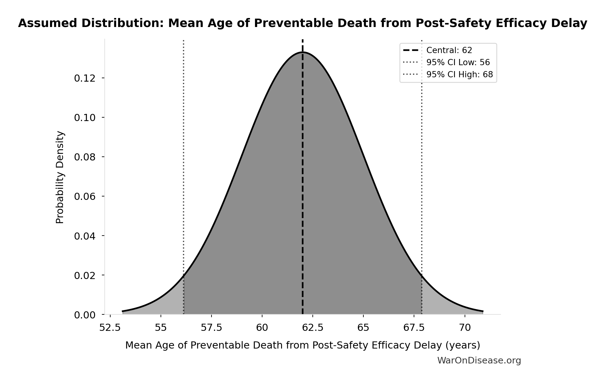
- Mean Age of Preventable Death from Post-Safety Efficacy Delay 📊: 62 years (SE: ±3 years)
\[ \begin{gathered} YLL_{lag} \\ = Deaths_{lag} \times (LE_{global} - Age_{death,delay}) \\ = 416M \times (79 - 62) \\ = 7.07B \end{gathered} \] where: \[ \begin{gathered} Deaths_{lag} \\ = T_{lag} \times Deaths_{disease,daily} \times 338 \\ = 8.2 \times 150{,}000 \times 338 \\ = 416M \end{gathered} \] ~ Medium confidence
Sensitivity Analysis
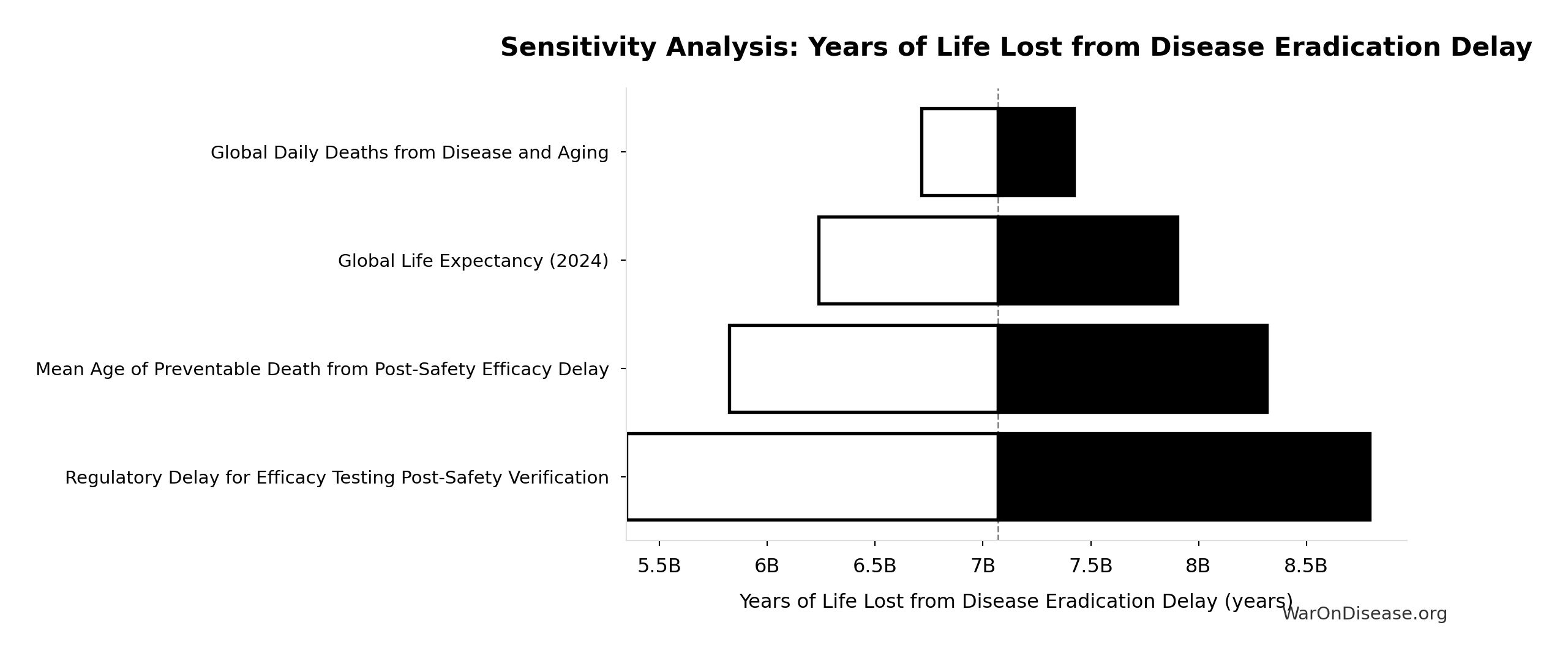
Sensitivity Indices for Years of Life Lost from Disease Eradication Delay
Regression-based sensitivity showing which inputs explain the most variance in the output.
| Input Parameter | Sensitivity Coefficient | Interpretation |
|---|---|---|
| Global Life Expectancy (2024) (years) | 2.0066 | Strong driver |
| Mean Age of Preventable Death from Post-Safety Efficacy Delay (years) | -1.3852 | Strong driver |
| Total Deaths from Disease Eradication Delay (deaths) | 0.3779 | Moderate driver |
Interpretation: Standardized coefficients show the change in output (in SD units) per 1 SD change in input. Values near ±1 indicate strong influence; values exceeding ±1 may occur with correlated inputs.
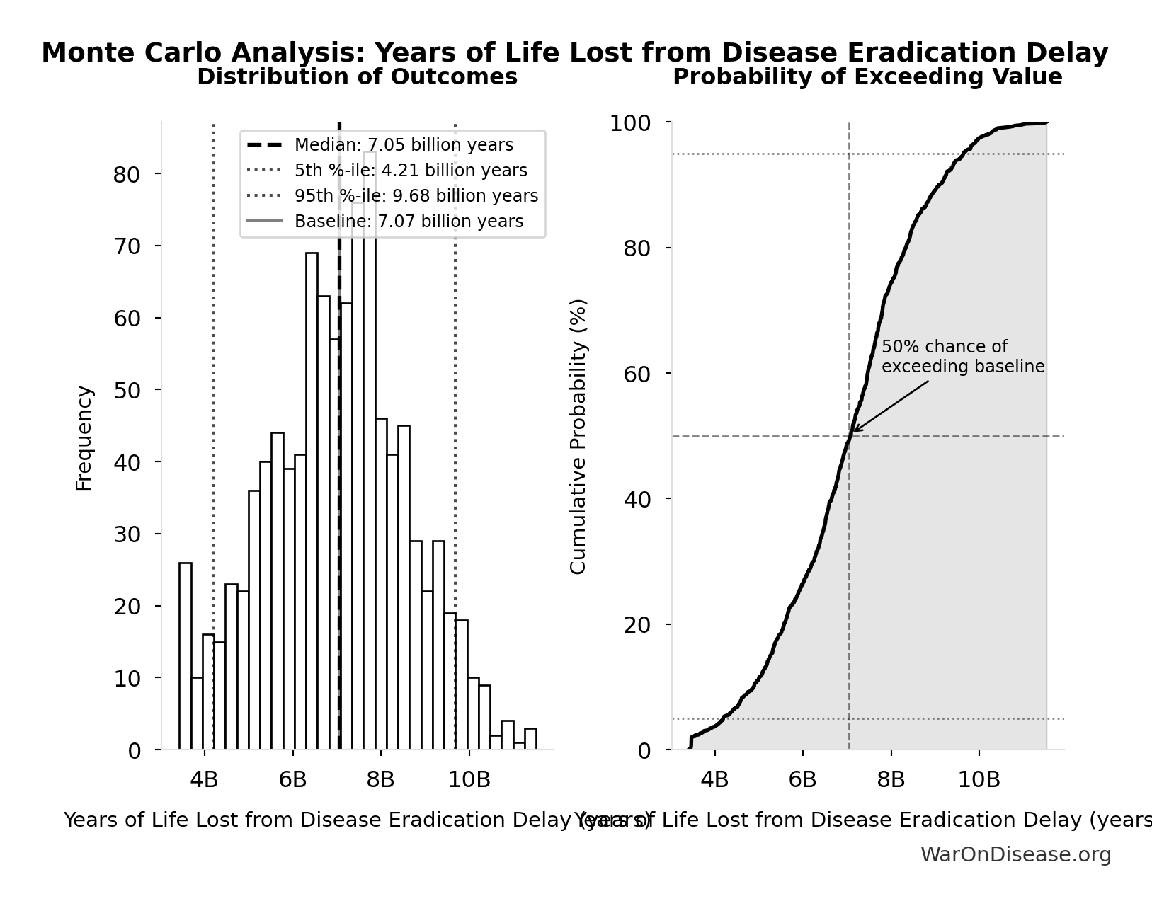
Monte Carlo Distribution
Simulation Results Summary: Years of Life Lost from Disease Eradication Delay
| Statistic | Value |
|---|---|
| Baseline (deterministic) | 7.07 billion |
| Mean (expected value) | 7.03 billion |
| Median (50th percentile) | 7.05 billion |
| Standard Deviation | 1.62 billion |
| 90% Range (5th-95th percentile) | [4.21 billion, 9.68 billion] |
The histogram shows the distribution of Years of Life Lost from Disease Eradication Delay across 10,000 Monte Carlo simulations. The CDF (right) shows the probability of the outcome exceeding any given value, which is useful for risk assessment.
Exceedance Probability
This exceedance probability chart shows the likelihood that Years of Life Lost from Disease Eradication Delay will exceed any given threshold. Higher curves indicate more favorable outcomes with greater certainty.
dFDA New Treatments Per Year: 185 diseases/year
Diseases per year receiving their first effective treatment with dFDA. Scales proportionally with trial capacity multiplier.
Inputs:
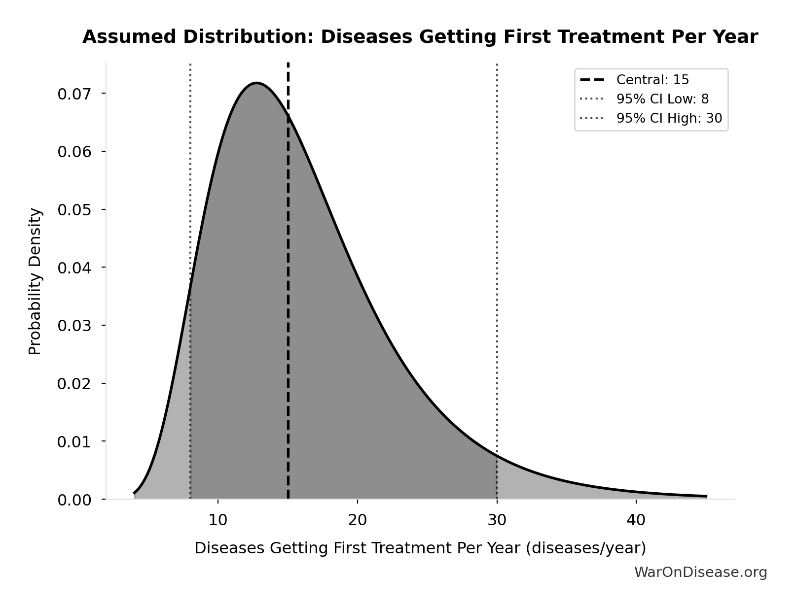
- Diseases Getting First Treatment Per Year 📊: 15 diseases/year (95% CI: 8 diseases/year - 30 diseases/year)
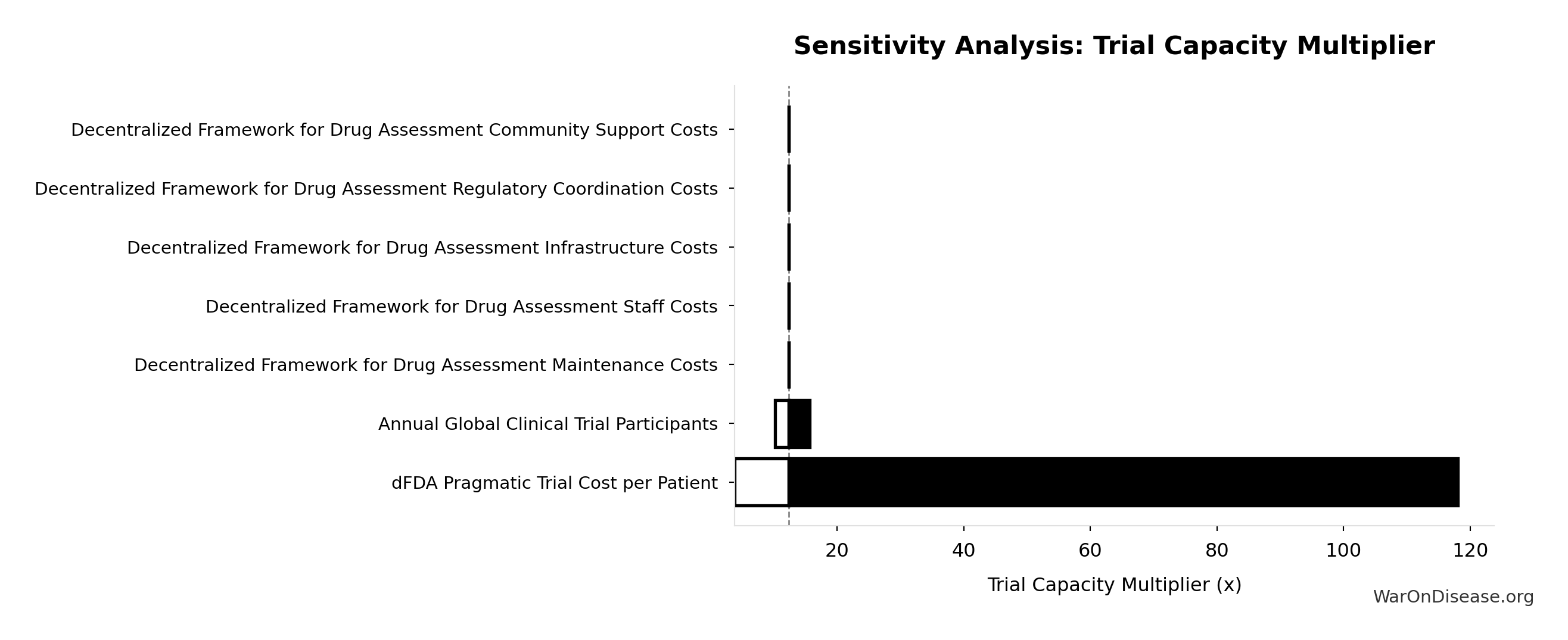
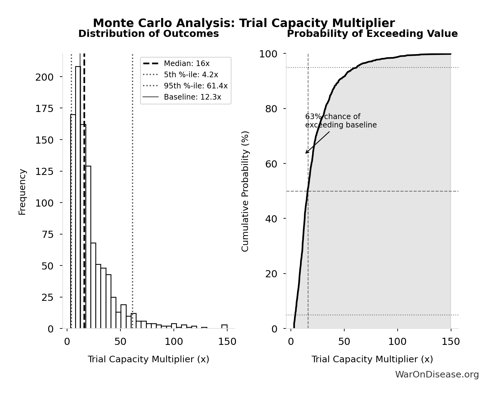
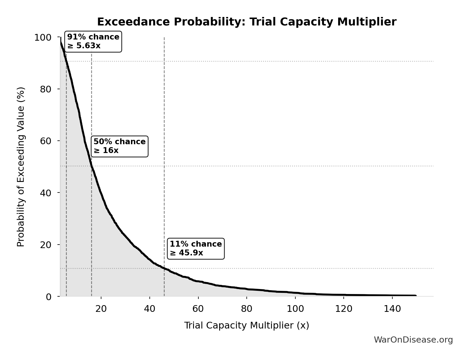
- Trial Capacity Multiplier 🔢: 12.3x
\[ \begin{gathered} Treatments_{dFDA,ann} \\ = Treatments_{new,ann} \times k_{capacity} \\ = 15 \times 12.3 \\ = 185 \end{gathered} \] where: \[ \begin{gathered} k_{capacity} \\ = \frac{N_{fundable,dFDA}}{Slots_{curr}} \\ = \frac{23.4M}{1.9M} \\ = 12.3 \end{gathered} \] where: \[ \begin{gathered} N_{fundable,dFDA} \\ = \frac{Subsidies_{dFDA,ann}}{Cost_{pragmatic,pt}} \\ = \frac{\$21.8B}{\$929} \\ = 23.4M \end{gathered} \] where: \[ \begin{gathered} Subsidies_{dFDA,ann} \\ = Funding_{dFDA,ann} - OPEX_{dFDA} \\ = \$21.8B - \$40M \\ = \$21.8B \end{gathered} \] where: \[ \begin{gathered} OPEX_{dFDA} \\ = Cost_{platform} + Cost_{staff} + Cost_{infra} \\ + Cost_{regulatory} + Cost_{community} \\ = \$15M + \$10M + \$8M + \$5M + \$2M \\ = \$40M \end{gathered} \] ? Low confidence
Sensitivity Analysis
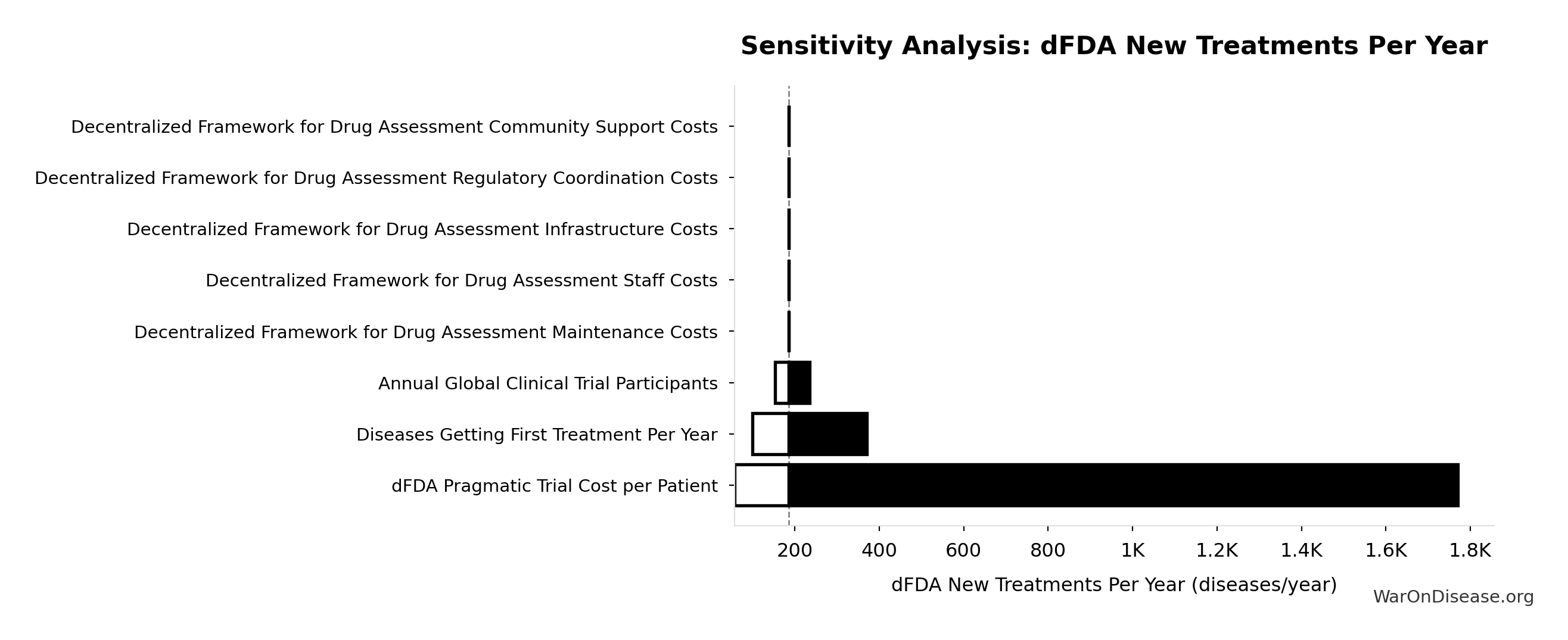
Sensitivity Indices for dFDA New Treatments Per Year
Regression-based sensitivity showing which inputs explain the most variance in the output.
| Input Parameter | Sensitivity Coefficient | Interpretation |
|---|---|---|
| Trial Capacity Multiplier (x) | 0.9380 | Strong driver |
| Diseases Getting First Treatment Per Year (diseases/year) | -0.0784 | Minimal effect |
Interpretation: Standardized coefficients show the change in output (in SD units) per 1 SD change in input. Values near ±1 indicate strong influence; values exceeding ±1 may occur with correlated inputs.
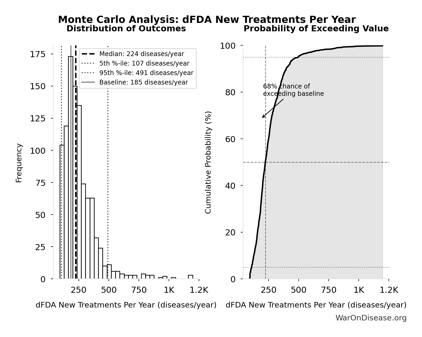
Monte Carlo Distribution
Simulation Results Summary: dFDA New Treatments Per Year
| Statistic | Value |
|---|---|
| Baseline (deterministic) | 185 |
| Mean (expected value) | 254 |
| Median (50th percentile) | 224 |
| Standard Deviation | 141 |
| 90% Range (5th-95th percentile) | [107, 491] |
The histogram shows the distribution of dFDA New Treatments Per Year across 10,000 Monte Carlo simulations. The CDF (right) shows the probability of the outcome exceeding any given value, which is useful for risk assessment.
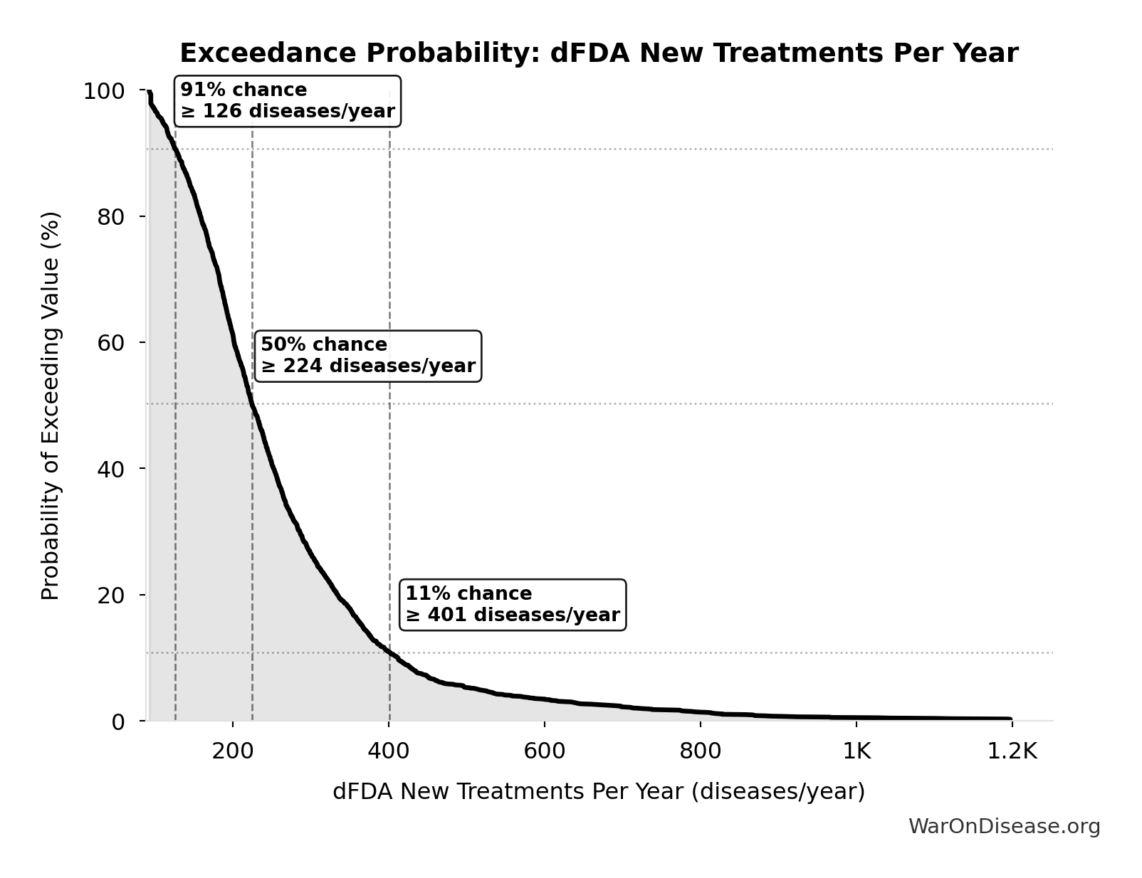
Exceedance Probability
This exceedance probability chart shows the likelihood that dFDA New Treatments Per Year will exceed any given threshold. Higher curves indicate more favorable outcomes with greater certainty.
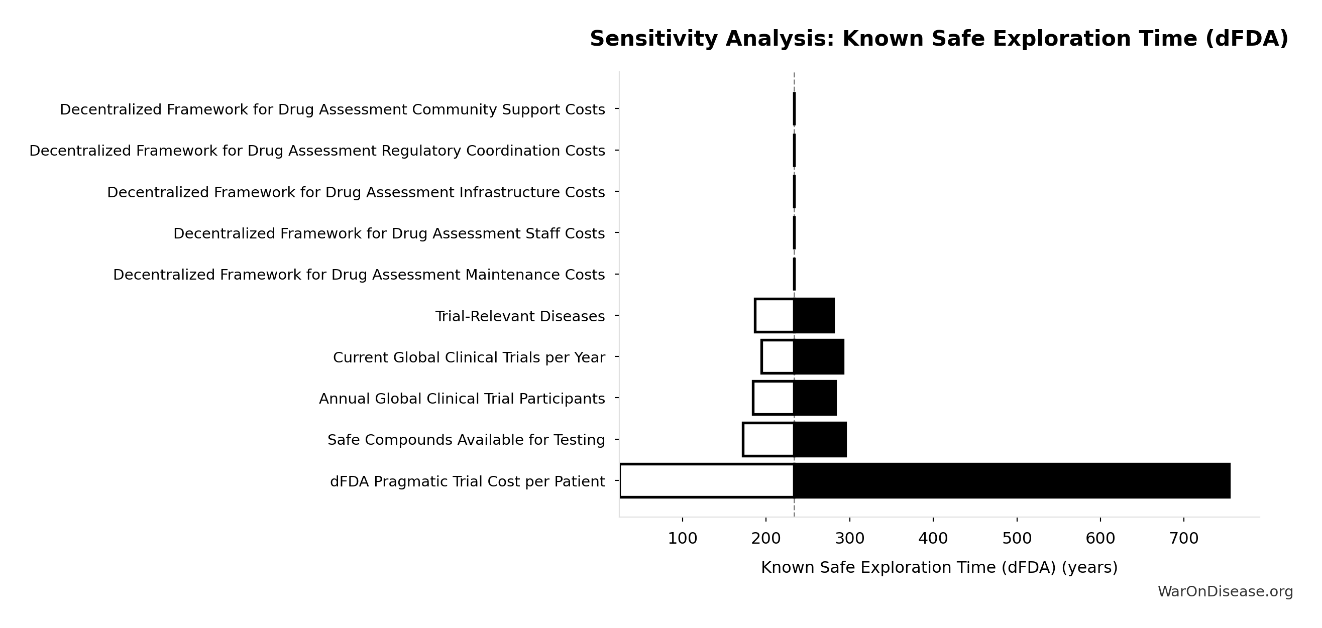
Known Safe Exploration Time (dFDA): 234 years
Years to test all known safe drug-disease combinations with dFDA trial capacity
Inputs:
- Possible Drug-Disease Combinations 🔢: 9.5 million combinations
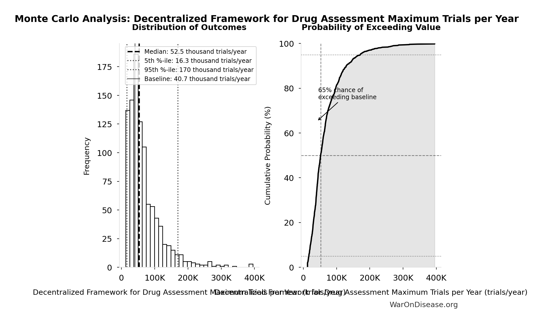
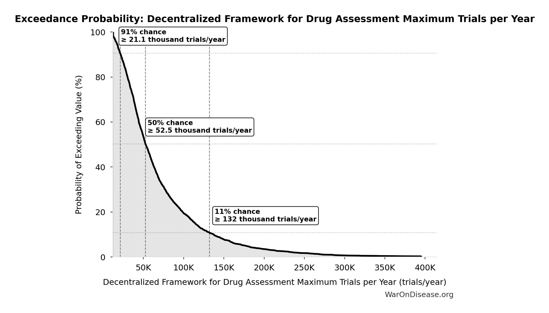
- Decentralized Framework for Drug Assessment Maximum Trials per Year 🔢: 40.7 thousand trials/year
\[ \begin{gathered} T_{safe,dFDA} \\ = \frac{N_{combos}}{Capacity_{trials}} \\ = \frac{9.5M}{40{,}700} \\ = 234 \end{gathered} \] where: \[ \begin{gathered} N_{combos} \\ = N_{safe} \times N_{diseases,trial} \\ = 9{,}500 \times 1{,}000 \\ = 9.5M \end{gathered} \] where: \[ \begin{gathered} Capacity_{trials} \\ = Trials_{ann,curr} \times k_{capacity} \\ = 3{,}300 \times 12.3 \\ = 40{,}700 \end{gathered} \] where: \[ \begin{gathered} k_{capacity} \\ = \frac{N_{fundable,dFDA}}{Slots_{curr}} \\ = \frac{23.4M}{1.9M} \\ = 12.3 \end{gathered} \] where: \[ \begin{gathered} N_{fundable,dFDA} \\ = \frac{Subsidies_{dFDA,ann}}{Cost_{pragmatic,pt}} \\ = \frac{\$21.8B}{\$929} \\ = 23.4M \end{gathered} \] where: \[ \begin{gathered} Subsidies_{dFDA,ann} \\ = Funding_{dFDA,ann} - OPEX_{dFDA} \\ = \$21.8B - \$40M \\ = \$21.8B \end{gathered} \] where: \[ \begin{gathered} OPEX_{dFDA} \\ = Cost_{platform} + Cost_{staff} + Cost_{infra} \\ + Cost_{regulatory} + Cost_{community} \\ = \$15M + \$10M + \$8M + \$5M + \$2M \\ = \$40M \end{gathered} \] ✓ High confidence
Sensitivity Analysis
Sensitivity Indices for Known Safe Exploration Time (dFDA)
Regression-based sensitivity showing which inputs explain the most variance in the output.
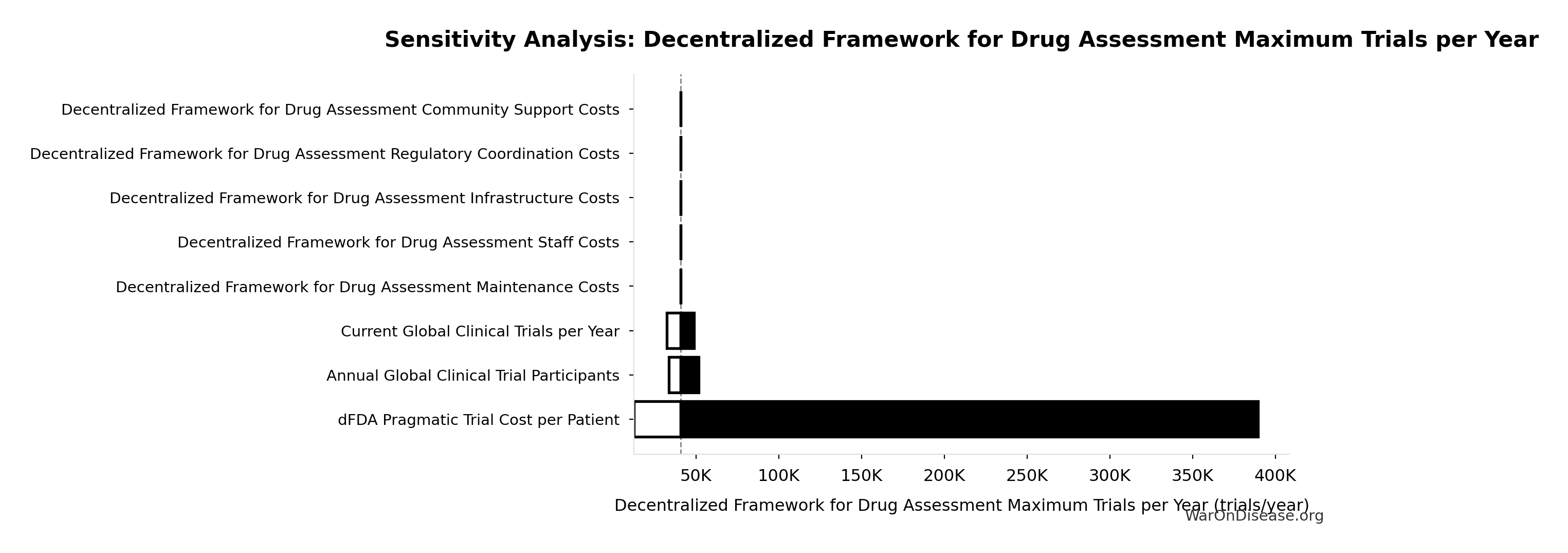
| Input Parameter | Sensitivity Coefficient | Interpretation |
|---|---|---|
| Decentralized Framework for Drug Assessment Maximum Trials per Year (trials/year) | -0.6771 | Strong driver |
Interpretation: Standardized coefficients show the change in output (in SD units) per 1 SD change in input. Values near ±1 indicate strong influence; values exceeding ±1 may occur with correlated inputs.
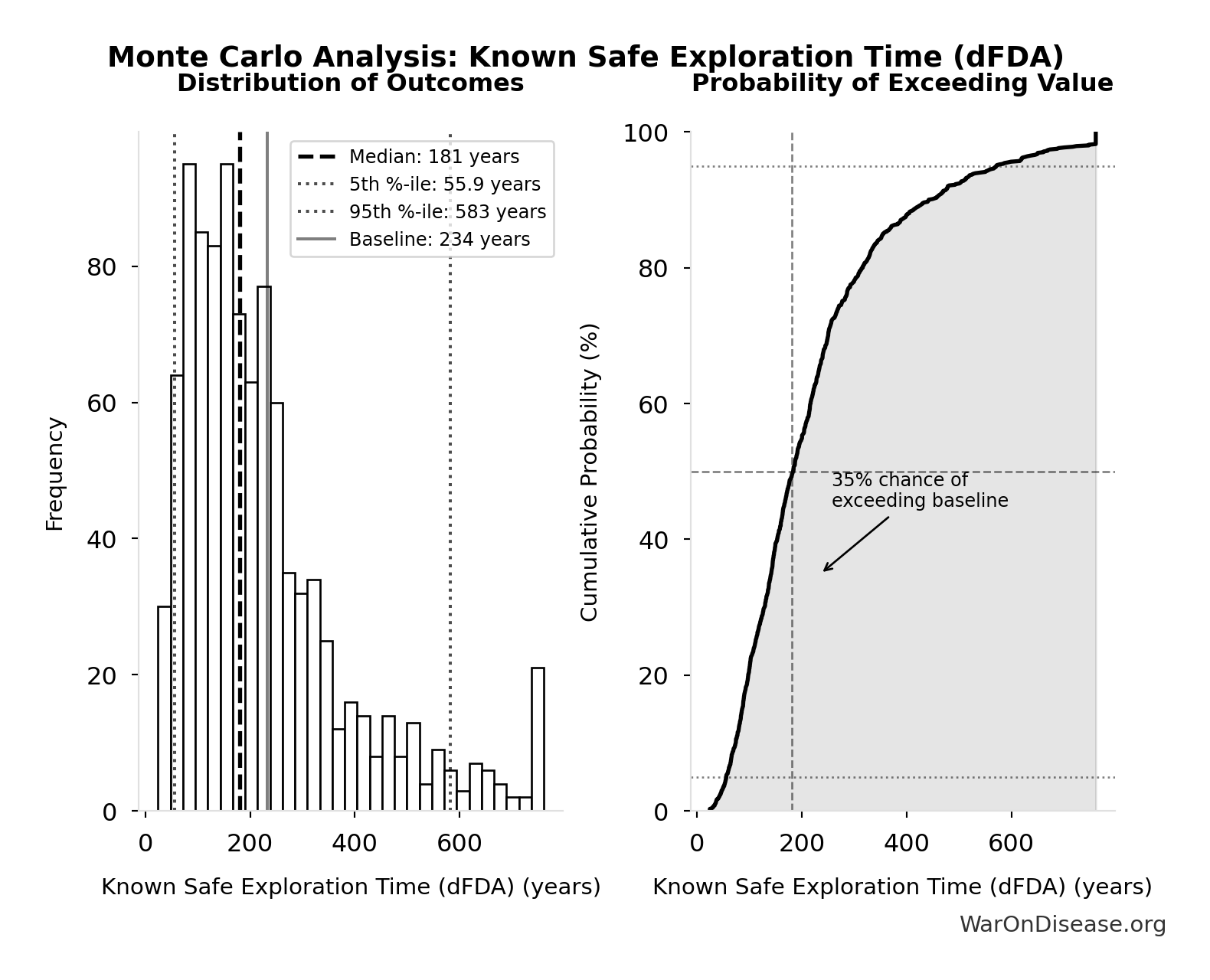
Monte Carlo Distribution
Simulation Results Summary: Known Safe Exploration Time (dFDA)
| Statistic | Value |
|---|---|
| Baseline (deterministic) | 234 |
| Mean (expected value) | 227 |
| Median (50th percentile) | 181 |
| Standard Deviation | 162 |
| 90% Range (5th-95th percentile) | [55.9, 583] |
The histogram shows the distribution of Known Safe Exploration Time (dFDA) across 10,000 Monte Carlo simulations. The CDF (right) shows the probability of the outcome exceeding any given value, which is useful for risk assessment.
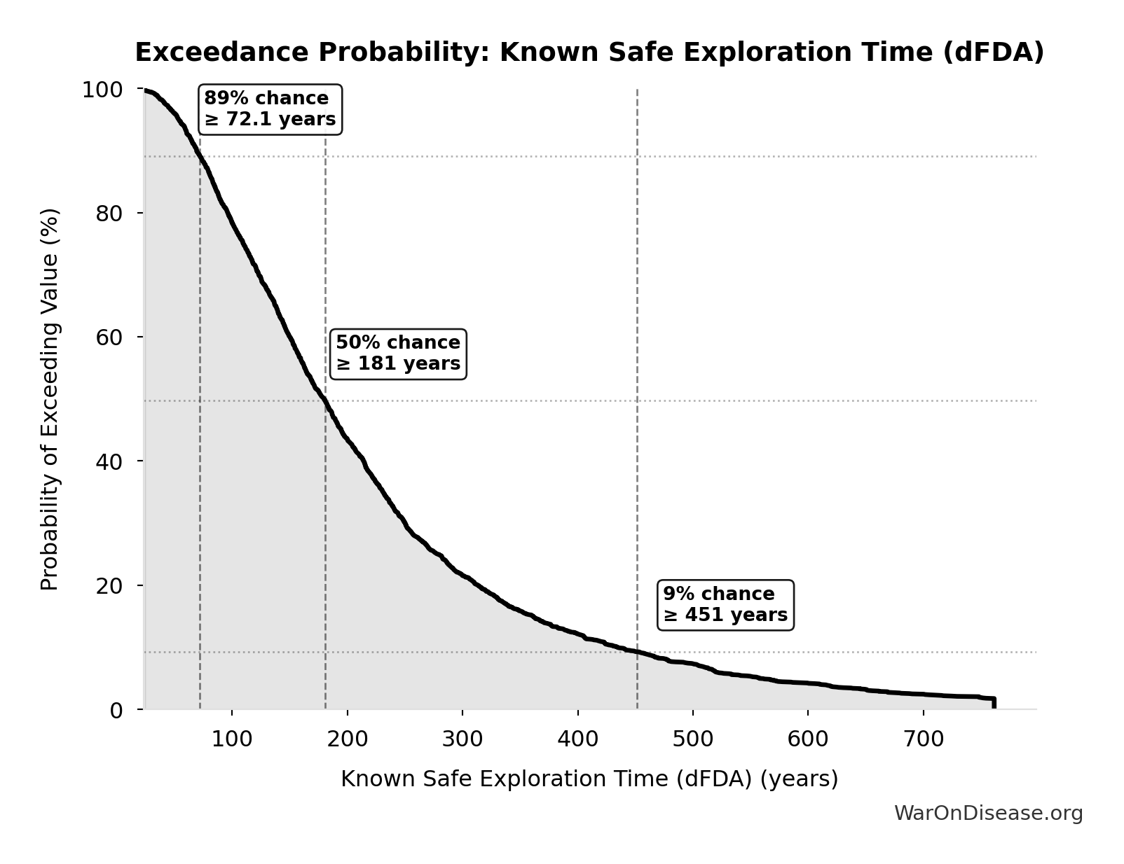
Exceedance Probability
This exceedance probability chart shows the likelihood that Known Safe Exploration Time (dFDA) will exceed any given threshold. Higher curves indicate more favorable outcomes with greater certainty.
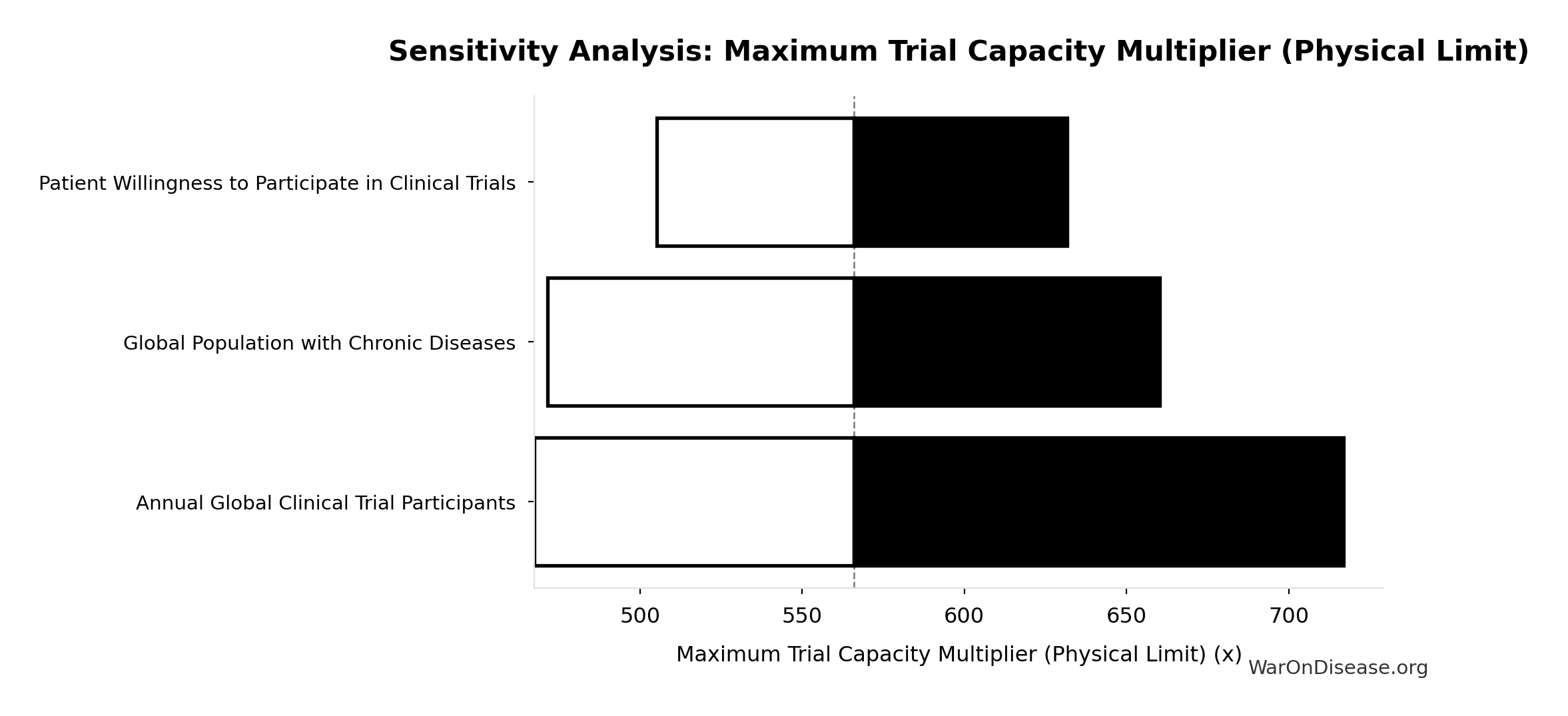
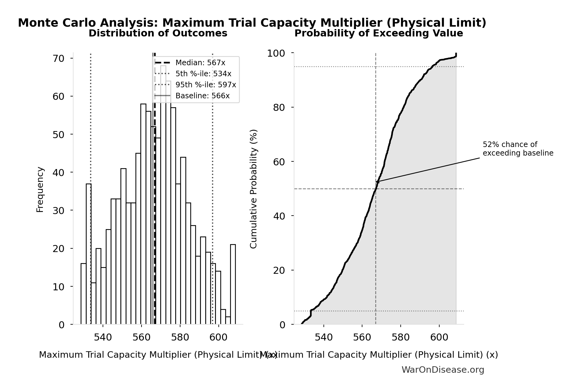
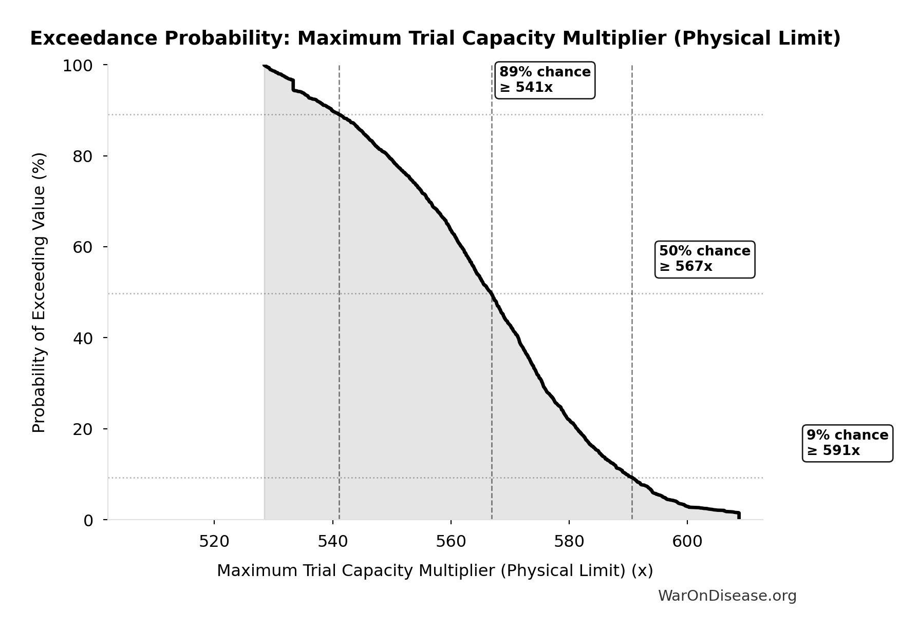
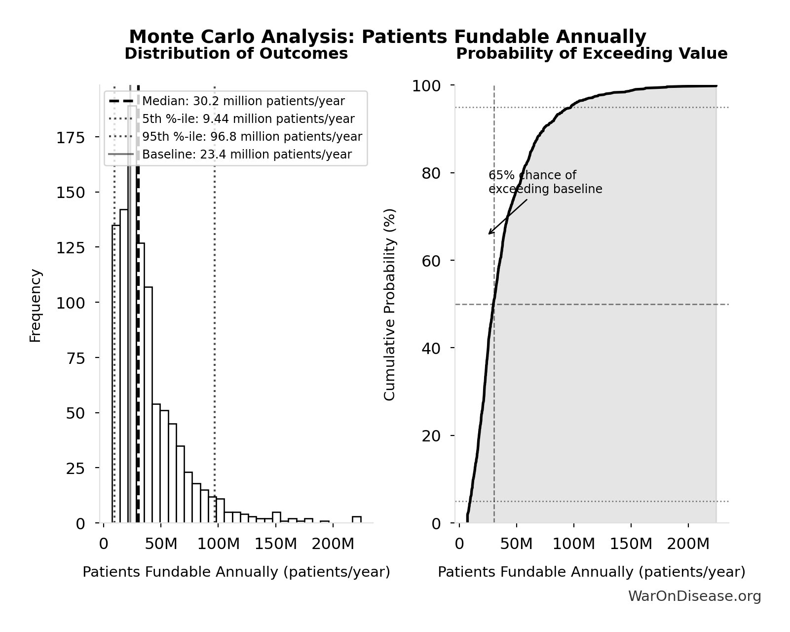
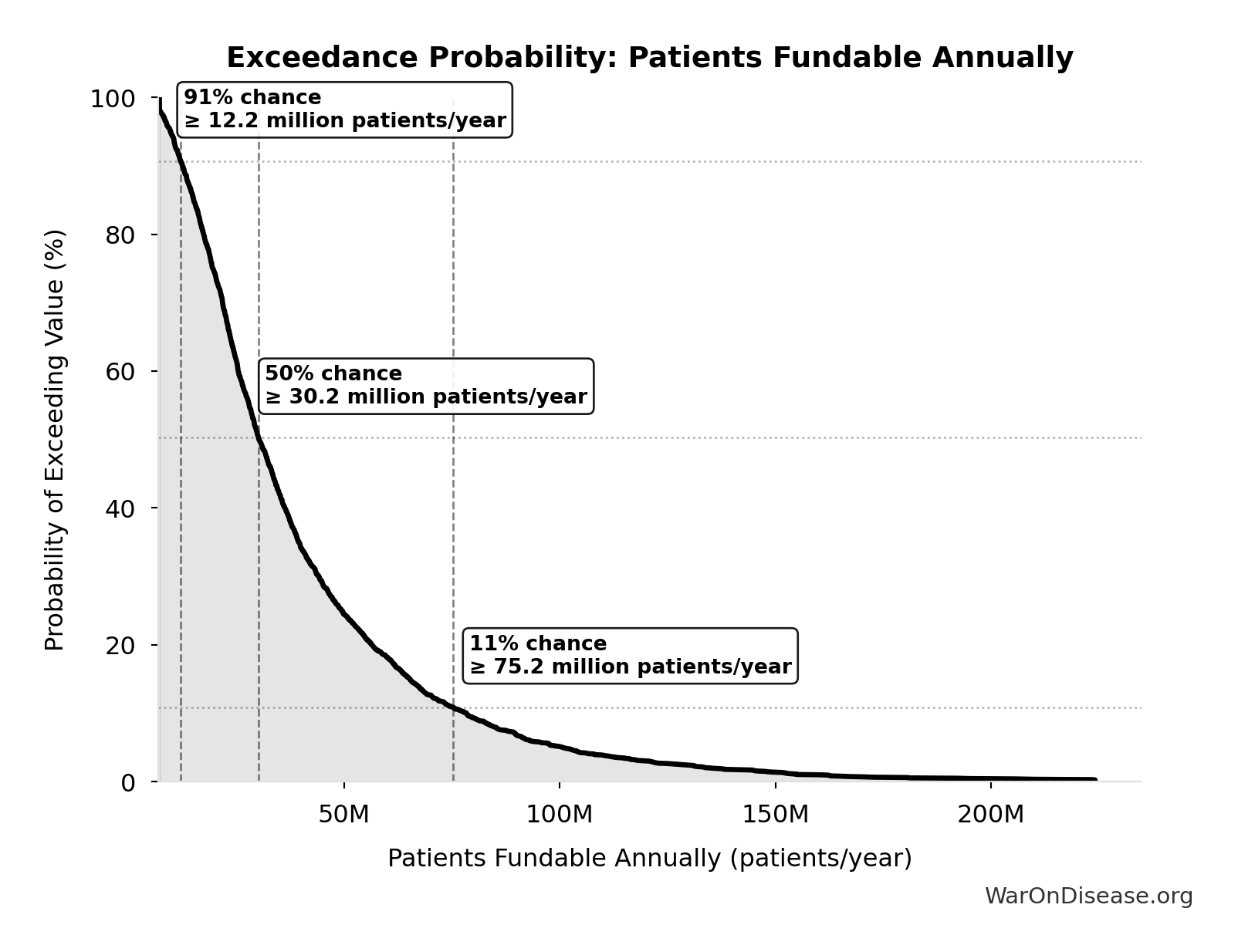
Maximum Trial Capacity Multiplier (Physical Limit): 566x
Physical upper bound on trial-capacity multiplier from participant availability. Even with unlimited funding, annual trial enrollment cannot exceed willing participant pool.
Inputs:
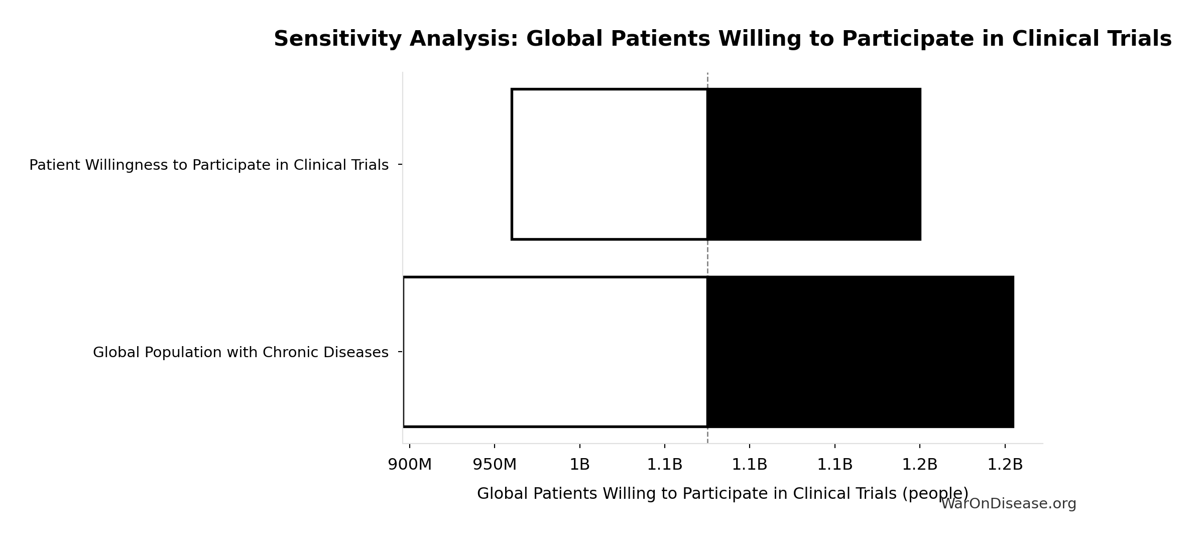
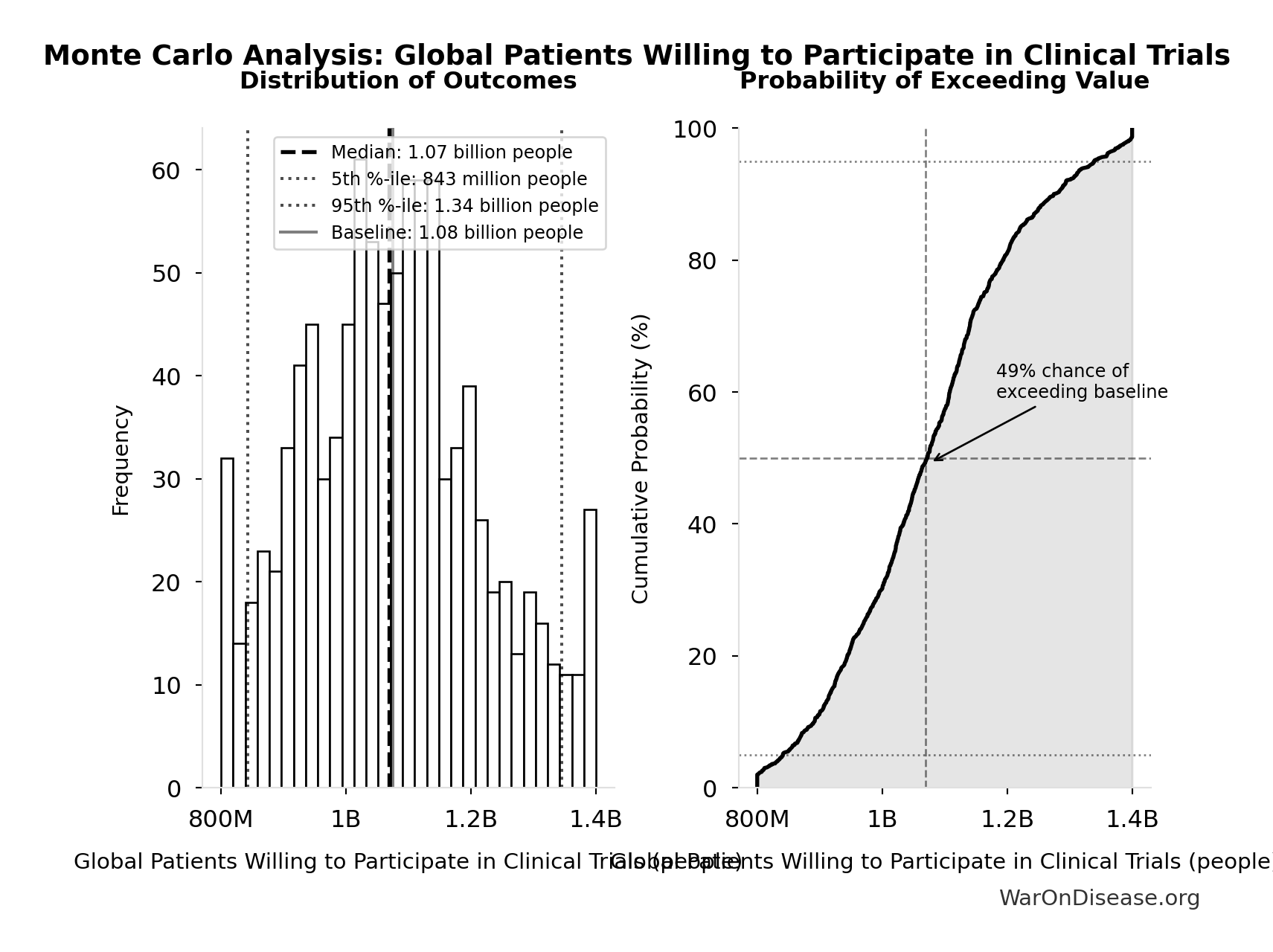
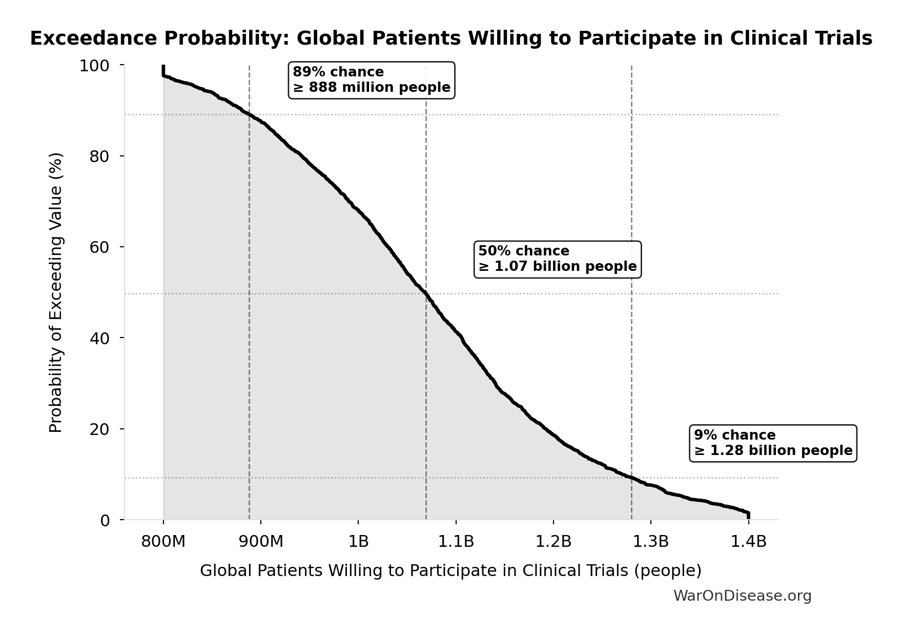
- Global Patients Willing to Participate in Clinical Trials 🔢: 1.08 billion people
- Annual Global Clinical Trial Participants 📊: 1.9 million patients/year (95% CI: 1.5 million patients/year - 2.3 million patients/year)
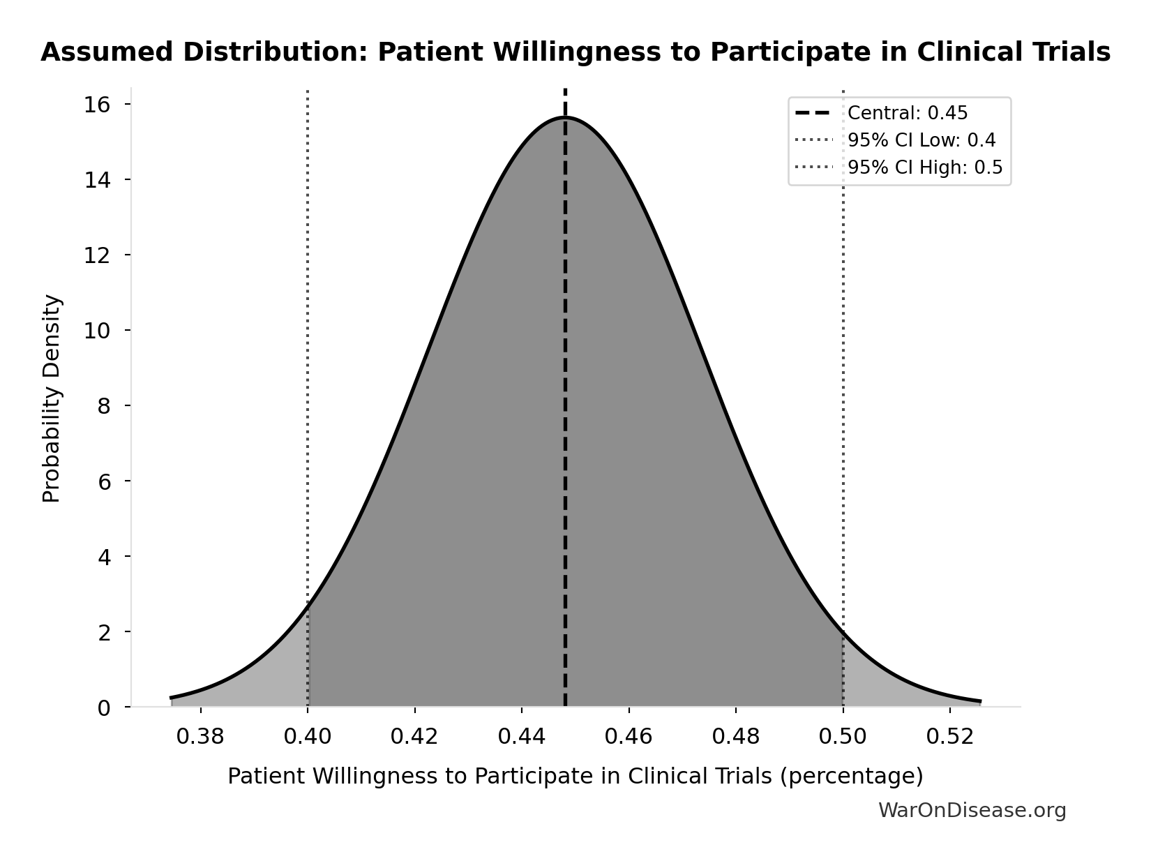
\[ \begin{gathered} k_{capacity,max} \\ = \frac{N_{willing}}{Slots_{curr}} \\ = \frac{1.08B}{1.9M} \\ = 566 \end{gathered} \] where: \[ \begin{gathered} N_{willing} \\ = N_{patients} \times Pct_{willing} \\ = 2.4B \times 44.8\% \\ = 1.08B \end{gathered} \] ~ Medium confidence
Sensitivity Analysis
Sensitivity Indices for Maximum Trial Capacity Multiplier (Physical Limit)
Regression-based sensitivity showing which inputs explain the most variance in the output.
| Input Parameter | Sensitivity Coefficient | Interpretation |
|---|---|---|
| Global Patients Willing to Participate in Clinical Trials (people) | 0.8980 | Strong driver |
| Annual Global Clinical Trial Participants (patients/year) | 0.0989 | Minimal effect |
Interpretation: Standardized coefficients show the change in output (in SD units) per 1 SD change in input. Values near ±1 indicate strong influence; values exceeding ±1 may occur with correlated inputs.
Monte Carlo Distribution
Simulation Results Summary: Maximum Trial Capacity Multiplier (Physical Limit)
| Statistic | Value |
|---|---|
| Baseline (deterministic) | 566x |
| Mean (expected value) | 567x |
| Median (50th percentile) | 567x |
| Standard Deviation | 18.4x |
| 90% Range (5th-95th percentile) | [534x, 597x] |
The histogram shows the distribution of Maximum Trial Capacity Multiplier (Physical Limit) across 10,000 Monte Carlo simulations. The CDF (right) shows the probability of the outcome exceeding any given value, which is useful for risk assessment.
Exceedance Probability
This exceedance probability chart shows the likelihood that Maximum Trial Capacity Multiplier (Physical Limit) will exceed any given threshold. Higher curves indicate more favorable outcomes with greater certainty.
Decentralized Framework for Drug Assessment Annual Net Savings (R&D Only): $58.6B
Annual net savings from R&D cost reduction only (gross savings minus operational costs, excludes regulatory delay value)
Inputs:
- Decentralized Framework for Drug Assessment Annual Benefit: R&D Savings 🔢: $58.6B
- Total Annual Decentralized Framework for Drug Assessment Operational Costs 🔢: $40M
\[ \begin{gathered} Savings_{RD,ann} \\ = Benefit_{RD,ann} - OPEX_{dFDA} \\ = \$58.6B - \$40M \\ = \$58.6B \end{gathered} \] where: \[ \begin{gathered} Benefit_{RD,ann} \\ = Spending_{trials} \times Reduce_{pct} \\ = \$60B \times 97.7\% \\ = \$58.6B \end{gathered} \] where: \[ \begin{gathered} Reduce_{pct} \\ = 1 - \frac{Cost_{pragmatic,pt}}{Cost_{P3,pt}} \\ = 1 - \frac{\$929}{\$41K} \\ = 97.7\% \end{gathered} \] where: \[ \begin{gathered} OPEX_{dFDA} \\ = Cost_{platform} + Cost_{staff} + Cost_{infra} \\ + Cost_{regulatory} + Cost_{community} \\ = \$15M + \$10M + \$8M + \$5M + \$2M \\ = \$40M \end{gathered} \] ✓ High confidence
Sensitivity Analysis
Sensitivity Indices for Decentralized Framework for Drug Assessment Annual Net Savings (R&D Only)
Regression-based sensitivity showing which inputs explain the most variance in the output.
| Input Parameter | Sensitivity Coefficient | Interpretation |
|---|---|---|
| Decentralized Framework for Drug Assessment Annual Benefit: R&D Savings (USD/year) | 1.0011 | Strong driver |
| Total Annual Decentralized Framework for Drug Assessment Operational Costs (USD/year) | -0.0011 | Minimal effect |
Interpretation: Standardized coefficients show the change in output (in SD units) per 1 SD change in input. Values near ±1 indicate strong influence; values exceeding ±1 may occur with correlated inputs.
Monte Carlo Distribution
Simulation Results Summary: Decentralized Framework for Drug Assessment Annual Net Savings (R&D Only)
| Statistic | Value |
|---|---|
| Baseline (deterministic) | $58.6B |
| Mean (expected value) | $58.8B |
| Median (50th percentile) | $57.8B |
| Standard Deviation | $7.66B |
| 90% Range (5th-95th percentile) | [$49.2B, $73B] |
The histogram shows the distribution of Decentralized Framework for Drug Assessment Annual Net Savings (R&D Only) across 10,000 Monte Carlo simulations. The CDF (right) shows the probability of the outcome exceeding any given value, which is useful for risk assessment.
Exceedance Probability
This exceedance probability chart shows the likelihood that Decentralized Framework for Drug Assessment Annual Net Savings (R&D Only) will exceed any given threshold. Higher curves indicate more favorable outcomes with greater certainty.
Decentralized Framework for Drug Assessment Total NPV Annual OPEX: $40M
Total NPV annual opex (Decentralized Framework for Drug Assessment core + DIH initiatives)
Inputs:
- Decentralized Framework for Drug Assessment Core framework Annual OPEX: $18.9M (95% CI: $11M - $26.5M)
- DIH Broader Initiatives Annual OPEX: $21.1M (95% CI: $14M - $32M)
\[ \begin{gathered} OPEX_{total} \\ = OPEX_{ann} + OPEX_{DIH,ann} \\ = \$18.9M + \$21.1M \\ = \$40M \end{gathered} \]
✓ High confidence
Sensitivity Analysis
Sensitivity Indices for Decentralized Framework for Drug Assessment Total NPV Annual OPEX
Regression-based sensitivity showing which inputs explain the most variance in the output.
| Input Parameter | Sensitivity Coefficient | Interpretation |
|---|---|---|
| DIH Broader Initiatives Annual OPEX (USD/year) | 0.5419 | Strong driver |
| Decentralized Framework for Drug Assessment Core framework Annual OPEX (USD/year) | 0.4592 | Moderate driver |
Interpretation: Standardized coefficients show the change in output (in SD units) per 1 SD change in input. Values near ±1 indicate strong influence; values exceeding ±1 may occur with correlated inputs.
Monte Carlo Distribution
Simulation Results Summary: Decentralized Framework for Drug Assessment Total NPV Annual OPEX
| Statistic | Value |
|---|---|
| Baseline (deterministic) | $40M |
| Mean (expected value) | $39.9M |
| Median (50th percentile) | $39.1M |
| Standard Deviation | $8.04M |
| 90% Range (5th-95th percentile) | [$27.5M, $55.4M] |
The histogram shows the distribution of Decentralized Framework for Drug Assessment Total NPV Annual OPEX across 10,000 Monte Carlo simulations. The CDF (right) shows the probability of the outcome exceeding any given value, which is useful for risk assessment.
Exceedance Probability
This exceedance probability chart shows the likelihood that Decentralized Framework for Drug Assessment Total NPV Annual OPEX will exceed any given threshold. Higher curves indicate more favorable outcomes with greater certainty.
NPV of Decentralized Framework for Drug Assessment Benefits (R&D Only, 10-Year Discounted): $389B
NPV of Decentralized Framework for Drug Assessment R&D savings only with 5-year adoption ramp (10-year horizon, most conservative financial estimate)
Inputs:
- Decentralized Framework for Drug Assessment Annual Net Savings (R&D Only) 🔢: $58.6B
- Standard Discount Rate for NPV Analysis: 3%
\[ \begin{gathered} NPV_{RD} \\ = \sum_{t=1}^{10} \frac{Savings_{RD,ann} \times \frac{\min(t,5)}{5}}{(1+r)^t} \end{gathered} \]
✓ High confidence
Sensitivity Analysis
Sensitivity Indices for NPV of Decentralized Framework for Drug Assessment Benefits (R&D Only, 10-Year Discounted)
Regression-based sensitivity showing which inputs explain the most variance in the output.
| Input Parameter | Sensitivity Coefficient | Interpretation |
|---|---|---|
| Decentralized Framework for Drug Assessment Annual Net Savings (R&D Only) (USD/year) | 1.0000 | Strong driver |
Interpretation: Standardized coefficients show the change in output (in SD units) per 1 SD change in input. Values near ±1 indicate strong influence; values exceeding ±1 may occur with correlated inputs.
Monte Carlo Distribution
Simulation Results Summary: NPV of Decentralized Framework for Drug Assessment Benefits (R&D Only, 10-Year Discounted)
| Statistic | Value |
|---|---|
| Baseline (deterministic) | $389B |
| Mean (expected value) | $391B |
| Median (50th percentile) | $384B |
| Standard Deviation | $50.9B |
| 90% Range (5th-95th percentile) | [$327B, $485B] |
The histogram shows the distribution of NPV of Decentralized Framework for Drug Assessment Benefits (R&D Only, 10-Year Discounted) across 10,000 Monte Carlo simulations. The CDF (right) shows the probability of the outcome exceeding any given value, which is useful for risk assessment.
Exceedance Probability
This exceedance probability chart shows the likelihood that NPV of Decentralized Framework for Drug Assessment Benefits (R&D Only, 10-Year Discounted) will exceed any given threshold. Higher curves indicate more favorable outcomes with greater certainty.
NPV Net Benefit (R&D Only): $389B
NPV net benefit using R&D savings only (benefits minus costs)
Inputs:
- NPV of Decentralized Framework for Drug Assessment Benefits (R&D Only, 10-Year Discounted) 🔢: $389B
- Decentralized Framework for Drug Assessment Total NPV Cost 🔢: $611M
\[ \begin{gathered} NPV_{net,RD} \\ = NPV_{RD} - Cost_{dFDA,total} \\ = \$389B - \$611M \\ = \$389B \end{gathered} \] where: \[ \begin{gathered} NPV_{RD} \\ = \sum_{t=1}^{10} \frac{Savings_{RD,ann} \times \frac{\min(t,5)}{5}}{(1+r)^t} \end{gathered} \] where: \[ \begin{gathered} Savings_{RD,ann} \\ = Benefit_{RD,ann} - OPEX_{dFDA} \\ = \$58.6B - \$40M \\ = \$58.6B \end{gathered} \] where: \[ \begin{gathered} Benefit_{RD,ann} \\ = Spending_{trials} \times Reduce_{pct} \\ = \$60B \times 97.7\% \\ = \$58.6B \end{gathered} \] where: \[ \begin{gathered} Reduce_{pct} \\ = 1 - \frac{Cost_{pragmatic,pt}}{Cost_{P3,pt}} \\ = 1 - \frac{\$929}{\$41K} \\ = 97.7\% \end{gathered} \] where: \[ \begin{gathered} OPEX_{dFDA} \\ = Cost_{platform} + Cost_{staff} + Cost_{infra} \\ + Cost_{regulatory} + Cost_{community} \\ = \$15M + \$10M + \$8M + \$5M + \$2M \\ = \$40M \end{gathered} \] where: \[ \begin{gathered} Cost_{dFDA,total} \\ = PV_{OPEX} + Cost_{upfront,total} \\ = \$342M + \$270M \\ = \$611M \end{gathered} \] where: \[ PV_{OPEX} = OPEX_{ann} \times \frac{1 - (1+r)^{-T}}{r} \] where: \[ \begin{gathered} OPEX_{total} \\ = OPEX_{ann} + OPEX_{DIH,ann} \\ = \$18.9M + \$21.1M \\ = \$40M \end{gathered} \] where: \[ \begin{gathered} Cost_{upfront,total} \\ = Cost_{upfront} + Cost_{DIH,init} \\ = \$40M + \$230M \\ = \$270M \end{gathered} \] ✓ High confidence
Sensitivity Analysis
Sensitivity Indices for NPV Net Benefit (R&D Only)
Regression-based sensitivity showing which inputs explain the most variance in the output.
| Input Parameter | Sensitivity Coefficient | Interpretation |
|---|---|---|
| NPV of Decentralized Framework for Drug Assessment Benefits (R&D Only, 10-Year Discounted) (USD) | 1.0025 | Strong driver |
| Decentralized Framework for Drug Assessment Total NPV Cost (USD) | -0.0025 | Minimal effect |
Interpretation: Standardized coefficients show the change in output (in SD units) per 1 SD change in input. Values near ±1 indicate strong influence; values exceeding ±1 may occur with correlated inputs.
Monte Carlo Distribution
Simulation Results Summary: NPV Net Benefit (R&D Only)
| Statistic | Value |
|---|---|
| Baseline (deterministic) | $389B |
| Mean (expected value) | $390B |
| Median (50th percentile) | $383B |
| Standard Deviation | $50.7B |
| 90% Range (5th-95th percentile) | [$326B, $484B] |
The histogram shows the distribution of NPV Net Benefit (R&D Only) across 10,000 Monte Carlo simulations. The CDF (right) shows the probability of the outcome exceeding any given value, which is useful for risk assessment.
Exceedance Probability
This exceedance probability chart shows the likelihood that NPV Net Benefit (R&D Only) will exceed any given threshold. Higher curves indicate more favorable outcomes with greater certainty.
Decentralized Framework for Drug Assessment Present Value of Annual OPEX Over 10 Years: $342M
Present value of annual opex over 10 years (NPV formula)
Inputs:
- Decentralized Framework for Drug Assessment Total NPV Annual OPEX 🔢: $40M
- Standard Discount Rate for NPV Analysis: 3%
- Standard Time Horizon for NPV Analysis: 10 years
\[ PV_{OPEX} = OPEX_{ann} \times \frac{1 - (1+r)^{-T}}{r} \]
✓ High confidence
Sensitivity Analysis
Sensitivity Indices for Decentralized Framework for Drug Assessment Present Value of Annual OPEX Over 10 Years
Regression-based sensitivity showing which inputs explain the most variance in the output.
| Input Parameter | Sensitivity Coefficient | Interpretation |
|---|---|---|
| Decentralized Framework for Drug Assessment Total NPV Annual OPEX (USD/year) | 1.0000 | Strong driver |
Interpretation: Standardized coefficients show the change in output (in SD units) per 1 SD change in input. Values near ±1 indicate strong influence; values exceeding ±1 may occur with correlated inputs.
Monte Carlo Distribution
Simulation Results Summary: Decentralized Framework for Drug Assessment Present Value of Annual OPEX Over 10 Years
| Statistic | Value |
|---|---|
| Baseline (deterministic) | $342M |
| Mean (expected value) | $340M |
| Median (50th percentile) | $333M |
| Standard Deviation | $68.6M |
| 90% Range (5th-95th percentile) | [$235M, $473M] |
The histogram shows the distribution of Decentralized Framework for Drug Assessment Present Value of Annual OPEX Over 10 Years across 10,000 Monte Carlo simulations. The CDF (right) shows the probability of the outcome exceeding any given value, which is useful for risk assessment.
Exceedance Probability
This exceedance probability chart shows the likelihood that Decentralized Framework for Drug Assessment Present Value of Annual OPEX Over 10 Years will exceed any given threshold. Higher curves indicate more favorable outcomes with greater certainty.
Decentralized Framework for Drug Assessment Total NPV Cost: $611M
Total NPV cost (upfront + PV of annual opex)
Inputs:
- Decentralized Framework for Drug Assessment Present Value of Annual OPEX Over 10 Years 🔢: $342M
- Decentralized Framework for Drug Assessment Total NPV Upfront Costs 🔢: $270M
\[ \begin{gathered} Cost_{dFDA,total} \\ = PV_{OPEX} + Cost_{upfront,total} \\ = \$342M + \$270M \\ = \$611M \end{gathered} \] where: \[ PV_{OPEX} = OPEX_{ann} \times \frac{1 - (1+r)^{-T}}{r} \] where: \[ \begin{gathered} OPEX_{total} \\ = OPEX_{ann} + OPEX_{DIH,ann} \\ = \$18.9M + \$21.1M \\ = \$40M \end{gathered} \] where: \[ \begin{gathered} Cost_{upfront,total} \\ = Cost_{upfront} + Cost_{DIH,init} \\ = \$40M + \$230M \\ = \$270M \end{gathered} \] ✓ High confidence
Sensitivity Analysis
Sensitivity Indices for Decentralized Framework for Drug Assessment Total NPV Cost
Regression-based sensitivity showing which inputs explain the most variance in the output.
| Input Parameter | Sensitivity Coefficient | Interpretation |
|---|---|---|
| Decentralized Framework for Drug Assessment Present Value of Annual OPEX Over 10 Years (USD) | 0.5417 | Strong driver |
| Decentralized Framework for Drug Assessment Total NPV Upfront Costs (USD) | 0.4585 | Moderate driver |
Interpretation: Standardized coefficients show the change in output (in SD units) per 1 SD change in input. Values near ±1 indicate strong influence; values exceeding ±1 may occur with correlated inputs.
Monte Carlo Distribution
Simulation Results Summary: Decentralized Framework for Drug Assessment Total NPV Cost
| Statistic | Value |
|---|---|
| Baseline (deterministic) | $611M |
| Mean (expected value) | $609M |
| Median (50th percentile) | $595M |
| Standard Deviation | $127M |
| 90% Range (5th-95th percentile) | [$415M, $853M] |
The histogram shows the distribution of Decentralized Framework for Drug Assessment Total NPV Cost across 10,000 Monte Carlo simulations. The CDF (right) shows the probability of the outcome exceeding any given value, which is useful for risk assessment.
Exceedance Probability
This exceedance probability chart shows the likelihood that Decentralized Framework for Drug Assessment Total NPV Cost will exceed any given threshold. Higher curves indicate more favorable outcomes with greater certainty.
Decentralized Framework for Drug Assessment Total NPV Upfront Costs: $270M
Total NPV upfront costs (Decentralized Framework for Drug Assessment core + DIH initiatives)
Inputs:
- Decentralized Framework for Drug Assessment Core framework Build Cost: $40M (95% CI: $25M - $65M)
- DIH Broader Initiatives Upfront Cost: $230M (95% CI: $150M - $350M)
\[ \begin{gathered} Cost_{upfront,total} \\ = Cost_{upfront} + Cost_{DIH,init} \\ = \$40M + \$230M \\ = \$270M \end{gathered} \]
✓ High confidence
Sensitivity Analysis
Sensitivity Indices for Decentralized Framework for Drug Assessment Total NPV Upfront Costs
Regression-based sensitivity showing which inputs explain the most variance in the output.
| Input Parameter | Sensitivity Coefficient | Interpretation |
|---|---|---|
| DIH Broader Initiatives Upfront Cost (USD) | 0.8338 | Strong driver |
| Decentralized Framework for Drug Assessment Core framework Build Cost (USD) | 0.1662 | Weak driver |
Interpretation: Standardized coefficients show the change in output (in SD units) per 1 SD change in input. Values near ±1 indicate strong influence; values exceeding ±1 may occur with correlated inputs.
Monte Carlo Distribution
Simulation Results Summary: Decentralized Framework for Drug Assessment Total NPV Upfront Costs
| Statistic | Value |
|---|---|
| Baseline (deterministic) | $270M |
| Mean (expected value) | $269M |
| Median (50th percentile) | $262M |
| Standard Deviation | $58.1M |
| 90% Range (5th-95th percentile) | [$181M, $380M] |
The histogram shows the distribution of Decentralized Framework for Drug Assessment Total NPV Upfront Costs across 10,000 Monte Carlo simulations. The CDF (right) shows the probability of the outcome exceeding any given value, which is useful for risk assessment.
Exceedance Probability
This exceedance probability chart shows the likelihood that Decentralized Framework for Drug Assessment Total NPV Upfront Costs will exceed any given threshold. Higher curves indicate more favorable outcomes with greater certainty.
Decentralized Framework for Drug Assessment Overhead Percentage of Treaty Funding: 0.147%
Percentage of treaty funding allocated to Decentralized Framework for Drug Assessment framework overhead
Inputs:
- Total Annual Decentralized Framework for Drug Assessment Operational Costs 🔢: $40M
- Annual Funding from 1% of Global Military Spending Redirected to DIH 🔢: $27.2B
\[ \begin{gathered} OPEX_{pct} \\ = \frac{OPEX_{dFDA}}{Funding_{treaty}} \\ = \frac{\$40M}{\$27.2B} \\ = 0.147\% \end{gathered} \] where: \[ \begin{gathered} OPEX_{dFDA} \\ = Cost_{platform} + Cost_{staff} + Cost_{infra} \\ + Cost_{regulatory} + Cost_{community} \\ = \$15M + \$10M + \$8M + \$5M + \$2M \\ = \$40M \end{gathered} \] where: \[ \begin{gathered} Funding_{treaty} \\ = Spending_{mil} \times Reduce_{treaty} \\ = \$2.72T \times 1\% \\ = \$27.2B \end{gathered} \] ✓ High confidence
Sensitivity Analysis
Sensitivity Indices for Decentralized Framework for Drug Assessment Overhead Percentage of Treaty Funding
Regression-based sensitivity showing which inputs explain the most variance in the output.
| Input Parameter | Sensitivity Coefficient | Interpretation |
|---|---|---|
| Total Annual Decentralized Framework for Drug Assessment Operational Costs (USD/year) | 1.0000 | Strong driver |
Interpretation: Standardized coefficients show the change in output (in SD units) per 1 SD change in input. Values near ±1 indicate strong influence; values exceeding ±1 may occur with correlated inputs.
Monte Carlo Distribution
Simulation Results Summary: Decentralized Framework for Drug Assessment Overhead Percentage of Treaty Funding
| Statistic | Value |
|---|---|
| Baseline (deterministic) | 0.147% |
| Mean (expected value) | 0.147% |
| Median (50th percentile) | 0.143% |
| Standard Deviation | 0.0302% |
| 90% Range (5th-95th percentile) | [0.1%, 0.204%] |
The histogram shows the distribution of Decentralized Framework for Drug Assessment Overhead Percentage of Treaty Funding across 10,000 Monte Carlo simulations. The CDF (right) shows the probability of the outcome exceeding any given value, which is useful for risk assessment.
Exceedance Probability
This exceedance probability chart shows the likelihood that Decentralized Framework for Drug Assessment Overhead Percentage of Treaty Funding will exceed any given threshold. Higher curves indicate more favorable outcomes with greater certainty.
dFDA Patients Fundable Annually: 23.4 million patients/year
Number of patients fundable annually from dFDA funding at pragmatic trial cost. Source-agnostic counterpart of DIH_PATIENTS_FUNDABLE_ANNUALLY.
Inputs:
- dFDA Annual Trial Subsidies 🔢: $21.8B
- dFDA Pragmatic Trial Cost per Patient 📊: $929 (95% CI: $97 - $3K)
\[ \begin{gathered} N_{fundable,dFDA} \\ = \frac{Subsidies_{dFDA,ann}}{Cost_{pragmatic,pt}} \\ = \frac{\$21.8B}{\$929} \\ = 23.4M \end{gathered} \] where: \[ \begin{gathered} Subsidies_{dFDA,ann} \\ = Funding_{dFDA,ann} - OPEX_{dFDA} \\ = \$21.8B - \$40M \\ = \$21.8B \end{gathered} \] where: \[ \begin{gathered} OPEX_{dFDA} \\ = Cost_{platform} + Cost_{staff} + Cost_{infra} \\ + Cost_{regulatory} + Cost_{community} \\ = \$15M + \$10M + \$8M + \$5M + \$2M \\ = \$40M \end{gathered} \] ✓ High confidence
Sensitivity Analysis
Sensitivity Indices for dFDA Patients Fundable Annually
Regression-based sensitivity showing which inputs explain the most variance in the output.
| Input Parameter | Sensitivity Coefficient | Interpretation |
|---|---|---|
| dFDA Annual Trial Subsidies (USD/year) | 2.3351 | Strong driver |
| dFDA Pragmatic Trial Cost per Patient (USD/patient) | 1.5755 | Strong driver |
Interpretation: Standardized coefficients show the change in output (in SD units) per 1 SD change in input. Values near ±1 indicate strong influence; values exceeding ±1 may occur with correlated inputs.
Monte Carlo Distribution
Simulation Results Summary: dFDA Patients Fundable Annually
| Statistic | Value |
|---|---|
| Baseline (deterministic) | 23.4 million |
| Mean (expected value) | 38.6 million |
| Median (50th percentile) | 30.2 million |
| Standard Deviation | 30.2 million |
| 90% Range (5th-95th percentile) | [9.46 million, 97 million] |
The histogram shows the distribution of dFDA Patients Fundable Annually across 10,000 Monte Carlo simulations. The CDF (right) shows the probability of the outcome exceeding any given value, which is useful for risk assessment.
Exceedance Probability
This exceedance probability chart shows the likelihood that dFDA Patients Fundable Annually will exceed any given threshold. Higher curves indicate more favorable outcomes with greater certainty.
dFDA Therapeutic Space Exploration Time: 36 years
Years to explore the entire therapeutic search space with dFDA implementation. At increased discovery rate, finding first treatments for all currently untreatable diseases takes ~36 years instead of ~443.
Inputs:
- Status Quo Therapeutic Space Exploration Time 🔢: 443 years
- Trial Capacity Multiplier 🔢: 12.3x
\[ \begin{gathered} T_{queue,dFDA} \\ = \frac{T_{queue,SQ}}{k_{capacity}} \\ = \frac{443}{12.3} \\ = 36 \end{gathered} \] where: \[ \begin{gathered} T_{queue,SQ} \\ = \frac{N_{untreated}}{Treatments_{new,ann}} \\ = \frac{6{,}650}{15} \\ = 443 \end{gathered} \] where: \[ \begin{gathered} N_{untreated} \\ = N_{rare} \times 0.95 \\ = 7{,}000 \times 0.95 \\ = 6{,}650 \end{gathered} \] where: \[ \begin{gathered} k_{capacity} \\ = \frac{N_{fundable,dFDA}}{Slots_{curr}} \\ = \frac{23.4M}{1.9M} \\ = 12.3 \end{gathered} \] where: \[ \begin{gathered} N_{fundable,dFDA} \\ = \frac{Subsidies_{dFDA,ann}}{Cost_{pragmatic,pt}} \\ = \frac{\$21.8B}{\$929} \\ = 23.4M \end{gathered} \] where: \[ \begin{gathered} Subsidies_{dFDA,ann} \\ = Funding_{dFDA,ann} - OPEX_{dFDA} \\ = \$21.8B - \$40M \\ = \$21.8B \end{gathered} \] where: \[ \begin{gathered} OPEX_{dFDA} \\ = Cost_{platform} + Cost_{staff} + Cost_{infra} \\ + Cost_{regulatory} + Cost_{community} \\ = \$15M + \$10M + \$8M + \$5M + \$2M \\ = \$40M \end{gathered} \] ? Low confidence
Sensitivity Analysis
Sensitivity Indices for dFDA Therapeutic Space Exploration Time
Regression-based sensitivity showing which inputs explain the most variance in the output.
| Input Parameter | Sensitivity Coefficient | Interpretation |
|---|---|---|
| Status Quo Therapeutic Space Exploration Time (years) | -1.3321 | Strong driver |
| Trial Capacity Multiplier (x) | 0.4867 | Moderate driver |
Interpretation: Standardized coefficients show the change in output (in SD units) per 1 SD change in input. Values near ±1 indicate strong influence; values exceeding ±1 may occur with correlated inputs.
Monte Carlo Distribution
Simulation Results Summary: dFDA Therapeutic Space Exploration Time
| Statistic | Value |
|---|---|
| Baseline (deterministic) | 36 |
| Mean (expected value) | 34.5 |
| Median (50th percentile) | 29.6 |
| Standard Deviation | 19.9 |
| 90% Range (5th-95th percentile) | [11.6, 77.1] |
The histogram shows the distribution of dFDA Therapeutic Space Exploration Time across 10,000 Monte Carlo simulations. The CDF (right) shows the probability of the outcome exceeding any given value, which is useful for risk assessment.
Exceedance Probability
This exceedance probability chart shows the likelihood that dFDA Therapeutic Space Exploration Time will exceed any given threshold. Higher curves indicate more favorable outcomes with greater certainty.
Daily R&D Savings from Trial Cost Reduction: $161M
Daily R&D savings from trial cost reduction (opportunity cost of delay)
Inputs:
\[ \begin{gathered} Savings_{RD,daily} \\ = Benefit_{RD,ann} \times 0.00274 \\ = \$58.6B \times 0.00274 \\ = \$161M \end{gathered} \] where: \[ \begin{gathered} Benefit_{RD,ann} \\ = Spending_{trials} \times Reduce_{pct} \\ = \$60B \times 97.7\% \\ = \$58.6B \end{gathered} \] where: \[ \begin{gathered} Reduce_{pct} \\ = 1 - \frac{Cost_{pragmatic,pt}}{Cost_{P3,pt}} \\ = 1 - \frac{\$929}{\$41K} \\ = 97.7\% \end{gathered} \] ✓ High confidence
Sensitivity Analysis
Sensitivity Indices for Daily R&D Savings from Trial Cost Reduction
Regression-based sensitivity showing which inputs explain the most variance in the output.
| Input Parameter | Sensitivity Coefficient | Interpretation |
|---|---|---|
| Decentralized Framework for Drug Assessment Annual Benefit: R&D Savings (USD/year) | 1.0000 | Strong driver |
Interpretation: Standardized coefficients show the change in output (in SD units) per 1 SD change in input. Values near ±1 indicate strong influence; values exceeding ±1 may occur with correlated inputs.
Monte Carlo Distribution
Simulation Results Summary: Daily R&D Savings from Trial Cost Reduction
| Statistic | Value |
|---|---|
| Baseline (deterministic) | $161M |
| Mean (expected value) | $161M |
| Median (50th percentile) | $158M |
| Standard Deviation | $21M |
| 90% Range (5th-95th percentile) | [$135M, $200M] |
The histogram shows the distribution of Daily R&D Savings from Trial Cost Reduction across 10,000 Monte Carlo simulations. The CDF (right) shows the probability of the outcome exceeding any given value, which is useful for risk assessment.
Exceedance Probability
This exceedance probability chart shows the likelihood that Daily R&D Savings from Trial Cost Reduction will exceed any given threshold. Higher curves indicate more favorable outcomes with greater certainty.
ROI from Decentralized Framework for Drug Assessment R&D Savings Only: 637:1
ROI from Decentralized Framework for Drug Assessment R&D savings only (10-year NPV, most conservative estimate)
Inputs:
- NPV of Decentralized Framework for Drug Assessment Benefits (R&D Only, 10-Year Discounted) 🔢: $389B
- Decentralized Framework for Drug Assessment Total NPV Cost 🔢: $611M
\[ \begin{gathered} ROI_{RD} \\ = \frac{NPV_{RD}}{Cost_{dFDA,total}} \\ = \frac{\$389B}{\$611M} \\ = 637 \end{gathered} \] where: \[ \begin{gathered} NPV_{RD} \\ = \sum_{t=1}^{10} \frac{Savings_{RD,ann} \times \frac{\min(t,5)}{5}}{(1+r)^t} \end{gathered} \] where: \[ \begin{gathered} Savings_{RD,ann} \\ = Benefit_{RD,ann} - OPEX_{dFDA} \\ = \$58.6B - \$40M \\ = \$58.6B \end{gathered} \] where: \[ \begin{gathered} Benefit_{RD,ann} \\ = Spending_{trials} \times Reduce_{pct} \\ = \$60B \times 97.7\% \\ = \$58.6B \end{gathered} \] where: \[ \begin{gathered} Reduce_{pct} \\ = 1 - \frac{Cost_{pragmatic,pt}}{Cost_{P3,pt}} \\ = 1 - \frac{\$929}{\$41K} \\ = 97.7\% \end{gathered} \] where: \[ \begin{gathered} OPEX_{dFDA} \\ = Cost_{platform} + Cost_{staff} + Cost_{infra} \\ + Cost_{regulatory} + Cost_{community} \\ = \$15M + \$10M + \$8M + \$5M + \$2M \\ = \$40M \end{gathered} \] where: \[ \begin{gathered} Cost_{dFDA,total} \\ = PV_{OPEX} + Cost_{upfront,total} \\ = \$342M + \$270M \\ = \$611M \end{gathered} \] where: \[ PV_{OPEX} = OPEX_{ann} \times \frac{1 - (1+r)^{-T}}{r} \] where: \[ \begin{gathered} OPEX_{total} \\ = OPEX_{ann} + OPEX_{DIH,ann} \\ = \$18.9M + \$21.1M \\ = \$40M \end{gathered} \] where: \[ \begin{gathered} Cost_{upfront,total} \\ = Cost_{upfront} + Cost_{DIH,init} \\ = \$40M + \$230M \\ = \$270M \end{gathered} \] ✓ High confidence
Sensitivity Analysis
Sensitivity Indices for ROI from Decentralized Framework for Drug Assessment R&D Savings Only
Regression-based sensitivity showing which inputs explain the most variance in the output.
| Input Parameter | Sensitivity Coefficient | Interpretation |
|---|---|---|
| Decentralized Framework for Drug Assessment Total NPV Cost (USD) | -2.6305 | Strong driver |
| NPV of Decentralized Framework for Drug Assessment Benefits (R&D Only, 10-Year Discounted) (USD) | 1.7615 | Strong driver |
Interpretation: Standardized coefficients show the change in output (in SD units) per 1 SD change in input. Values near ±1 indicate strong influence; values exceeding ±1 may occur with correlated inputs.
Monte Carlo Distribution
Simulation Results Summary: ROI from Decentralized Framework for Drug Assessment R&D Savings Only
| Statistic | Value |
|---|---|
| Baseline (deterministic) | 637:1 |
| Mean (expected value) | 653:1 |
| Median (50th percentile) | 645:1 |
| Standard Deviation | 58.4:1 |
| 90% Range (5th-95th percentile) | [569:1, 790:1] |
The histogram shows the distribution of ROI from Decentralized Framework for Drug Assessment R&D Savings Only across 10,000 Monte Carlo simulations. The CDF (right) shows the probability of the outcome exceeding any given value, which is useful for risk assessment.
Exceedance Probability
This exceedance probability chart shows the likelihood that ROI from Decentralized Framework for Drug Assessment R&D Savings Only will exceed any given threshold. Higher curves indicate more favorable outcomes with greater certainty.
Decentralized Framework for Drug Assessment Maximum Trials per Year: 40.7 thousand trials/year
Maximum trials per year possible with trial capacity multiplier
Inputs:
- Current Global Clinical Trials per Year 📊: 3.3 thousand trials/year (95% CI: 2.64 thousand trials/year - 3.96 thousand trials/year)
- Trial Capacity Multiplier 🔢: 12.3x
\[ \begin{gathered} Capacity_{trials} \\ = Trials_{ann,curr} \times k_{capacity} \\ = 3{,}300 \times 12.3 \\ = 40{,}700 \end{gathered} \] where: \[ \begin{gathered} k_{capacity} \\ = \frac{N_{fundable,dFDA}}{Slots_{curr}} \\ = \frac{23.4M}{1.9M} \\ = 12.3 \end{gathered} \] where: \[ \begin{gathered} N_{fundable,dFDA} \\ = \frac{Subsidies_{dFDA,ann}}{Cost_{pragmatic,pt}} \\ = \frac{\$21.8B}{\$929} \\ = 23.4M \end{gathered} \] where: \[ \begin{gathered} Subsidies_{dFDA,ann} \\ = Funding_{dFDA,ann} - OPEX_{dFDA} \\ = \$21.8B - \$40M \\ = \$21.8B \end{gathered} \] where: \[ \begin{gathered} OPEX_{dFDA} \\ = Cost_{platform} + Cost_{staff} + Cost_{infra} \\ + Cost_{regulatory} + Cost_{community} \\ = \$15M + \$10M + \$8M + \$5M + \$2M \\ = \$40M \end{gathered} \] ✓ High confidence
Sensitivity Analysis
Sensitivity Indices for Decentralized Framework for Drug Assessment Maximum Trials per Year
Regression-based sensitivity showing which inputs explain the most variance in the output.
| Input Parameter | Sensitivity Coefficient | Interpretation |
|---|---|---|
| Trial Capacity Multiplier (x) | 0.9321 | Strong driver |
| Current Global Clinical Trials per Year (trials/year) | -0.0802 | Minimal effect |
Interpretation: Standardized coefficients show the change in output (in SD units) per 1 SD change in input. Values near ±1 indicate strong influence; values exceeding ±1 may occur with correlated inputs.
Monte Carlo Distribution
Simulation Results Summary: Decentralized Framework for Drug Assessment Maximum Trials per Year
| Statistic | Value |
|---|---|
| Baseline (deterministic) | 40.7 thousand |
| Mean (expected value) | 67.4 thousand |
| Median (50th percentile) | 52.5 thousand |
| Standard Deviation | 53.2 thousand |
| 90% Range (5th-95th percentile) | [16.3 thousand, 170 thousand] |
The histogram shows the distribution of Decentralized Framework for Drug Assessment Maximum Trials per Year across 10,000 Monte Carlo simulations. The CDF (right) shows the probability of the outcome exceeding any given value, which is useful for risk assessment.
Exceedance Probability
This exceedance probability chart shows the likelihood that Decentralized Framework for Drug Assessment Maximum Trials per Year will exceed any given threshold. Higher curves indicate more favorable outcomes with greater certainty.
Trial Capacity Multiplier: 12.3x
Trial capacity multiplier from dFDA funding capacity vs. current global trial participation
Inputs:
- Annual Global Clinical Trial Participants 📊: 1.9 million patients/year (95% CI: 1.5 million patients/year - 2.3 million patients/year)
- dFDA Patients Fundable Annually 🔢: 23.4 million patients/year
\[ \begin{gathered} k_{capacity} \\ = \frac{N_{fundable,dFDA}}{Slots_{curr}} \\ = \frac{23.4M}{1.9M} \\ = 12.3 \end{gathered} \] where: \[ \begin{gathered} N_{fundable,dFDA} \\ = \frac{Subsidies_{dFDA,ann}}{Cost_{pragmatic,pt}} \\ = \frac{\$21.8B}{\$929} \\ = 23.4M \end{gathered} \] where: \[ \begin{gathered} Subsidies_{dFDA,ann} \\ = Funding_{dFDA,ann} - OPEX_{dFDA} \\ = \$21.8B - \$40M \\ = \$21.8B \end{gathered} \] where: \[ \begin{gathered} OPEX_{dFDA} \\ = Cost_{platform} + Cost_{staff} + Cost_{infra} \\ + Cost_{regulatory} + Cost_{community} \\ = \$15M + \$10M + \$8M + \$5M + \$2M \\ = \$40M \end{gathered} \] ✓ High confidence
Sensitivity Analysis
Sensitivity Indices for Trial Capacity Multiplier
Regression-based sensitivity showing which inputs explain the most variance in the output.
| Input Parameter | Sensitivity Coefficient | Interpretation |
|---|---|---|
| dFDA Patients Fundable Annually (patients/year) | 1.0768 | Strong driver |
| Annual Global Clinical Trial Participants (patients/year) | 0.0910 | Minimal effect |
Interpretation: Standardized coefficients show the change in output (in SD units) per 1 SD change in input. Values near ±1 indicate strong influence; values exceeding ±1 may occur with correlated inputs.
Monte Carlo Distribution
Simulation Results Summary: Trial Capacity Multiplier
| Statistic | Value |
|---|---|
| Baseline (deterministic) | 12.3x |
| Mean (expected value) | 22.1x |
| Median (50th percentile) | 16x |
| Standard Deviation | 20.2x |
| 90% Range (5th-95th percentile) | [4.2x, 61.4x] |
The histogram shows the distribution of Trial Capacity Multiplier across 10,000 Monte Carlo simulations. The CDF (right) shows the probability of the outcome exceeding any given value, which is useful for risk assessment.
Exceedance Probability
This exceedance probability chart shows the likelihood that Trial Capacity Multiplier will exceed any given threshold. Higher curves indicate more favorable outcomes with greater certainty.
Total DALYs from Elimination of Efficacy Lag Plus Earlier Treatment Discovery from Higher Trial Throughput: 565 billion DALYs
Total DALYs averted from the combined dFDA timeline shift. Calculated as annual global DALY burden × eventually avoidable percentage × timeline shift years. Includes both fatal and non-fatal diseases (WHO GBD methodology).
Inputs:
- Global Annual DALY Burden 📊: 2.88 billion DALYs/year (SE: ±150 million DALYs/year)
- Eventually Avoidable DALY Percentage: 92.6% (95% CI: 50% - 98%)
- dFDA Average Total Timeline Shift 🔢: 212 years
\[ \begin{gathered} DALYs_{max} \\ = DALYs_{global,ann} \times Pct_{avoid,DALY} \times T_{accel,max} \\ = 2.88B \times 92.6\% \times 212 \\ = 565B \end{gathered} \] where: \[ T_{accel,max} = T_{accel} + T_{lag} = 204 + 8.2 = 212 \] where: \[ \begin{gathered} T_{accel} \\ = T_{first,SQ} \times \left(1 - \frac{1}{k_{capacity}}\right) \\ = 222 \times \left(1 - \frac{1}{12.3}\right) \\ = 204 \end{gathered} \] where: \[ \begin{gathered} T_{first,SQ} \\ = T_{queue,SQ} \times 0.5 \\ = 443 \times 0.5 \\ = 222 \end{gathered} \] where: \[ \begin{gathered} T_{queue,SQ} \\ = \frac{N_{untreated}}{Treatments_{new,ann}} \\ = \frac{6{,}650}{15} \\ = 443 \end{gathered} \] where: \[ \begin{gathered} N_{untreated} \\ = N_{rare} \times 0.95 \\ = 7{,}000 \times 0.95 \\ = 6{,}650 \end{gathered} \] where: \[ \begin{gathered} k_{capacity} \\ = \frac{N_{fundable,dFDA}}{Slots_{curr}} \\ = \frac{23.4M}{1.9M} \\ = 12.3 \end{gathered} \] where: \[ \begin{gathered} N_{fundable,dFDA} \\ = \frac{Subsidies_{dFDA,ann}}{Cost_{pragmatic,pt}} \\ = \frac{\$21.8B}{\$929} \\ = 23.4M \end{gathered} \] where: \[ \begin{gathered} Subsidies_{dFDA,ann} \\ = Funding_{dFDA,ann} - OPEX_{dFDA} \\ = \$21.8B - \$40M \\ = \$21.8B \end{gathered} \] where: \[ \begin{gathered} OPEX_{dFDA} \\ = Cost_{platform} + Cost_{staff} + Cost_{infra} \\ + Cost_{regulatory} + Cost_{community} \\ = \$15M + \$10M + \$8M + \$5M + \$2M \\ = \$40M \end{gathered} \] ? Low confidence
Sensitivity Analysis
Sensitivity Indices for Total DALYs from Elimination of Efficacy Lag Plus Earlier Treatment Discovery from Higher Trial Throughput
Regression-based sensitivity showing which inputs explain the most variance in the output.
| Input Parameter | Sensitivity Coefficient | Interpretation |
|---|---|---|
| dFDA Average Total Timeline Shift (years) | 0.8999 | Strong driver |
| Eventually Avoidable DALY Percentage (percentage) | 0.4866 | Moderate driver |
| Global Annual DALY Burden (DALYs/year) | 0.0432 | Minimal effect |
Interpretation: Standardized coefficients show the change in output (in SD units) per 1 SD change in input. Values near ±1 indicate strong influence; values exceeding ±1 may occur with correlated inputs.
Monte Carlo Distribution
Simulation Results Summary: Total DALYs from Elimination of Efficacy Lag Plus Earlier Treatment Discovery from Higher Trial Throughput
| Statistic | Value |
|---|---|
| Baseline (deterministic) | 565 billion |
| Mean (expected value) | 610 billion |
| Median (50th percentile) | 614 billion |
| Standard Deviation | 148 billion |
| 90% Range (5th-95th percentile) | [361 billion, 877 billion] |
The histogram shows the distribution of Total DALYs from Elimination of Efficacy Lag Plus Earlier Treatment Discovery from Higher Trial Throughput across 10,000 Monte Carlo simulations. The CDF (right) shows the probability of the outcome exceeding any given value, which is useful for risk assessment.
Exceedance Probability
This exceedance probability chart shows the likelihood that Total DALYs from Elimination of Efficacy Lag Plus Earlier Treatment Discovery from Higher Trial Throughput will exceed any given threshold. Higher curves indicate more favorable outcomes with greater certainty.
Total Economic Benefit from Elimination of Efficacy Lag Plus Earlier Treatment Discovery from Higher Trial Throughput: $84.8 quadrillion
Total economic value from the combined dFDA timeline shift. DALYs valued at standard economic rate.
Inputs:
- Total DALYs from Elimination of Efficacy Lag Plus Earlier Treatment Discovery from Higher Trial Throughput 🔢: 565 billion DALYs
- Standard Economic Value per QALY 📊: $150K (SE: ±$30K)
\[ \begin{gathered} Value_{max} \\ = DALYs_{max} \times Value_{QALY} \\ = 565B \times \$150K \\ = \$84800T \end{gathered} \] where: \[ \begin{gathered} DALYs_{max} \\ = DALYs_{global,ann} \times Pct_{avoid,DALY} \times T_{accel,max} \\ = 2.88B \times 92.6\% \times 212 \\ = 565B \end{gathered} \] where: \[ T_{accel,max} = T_{accel} + T_{lag} = 204 + 8.2 = 212 \] where: \[ \begin{gathered} T_{accel} \\ = T_{first,SQ} \times \left(1 - \frac{1}{k_{capacity}}\right) \\ = 222 \times \left(1 - \frac{1}{12.3}\right) \\ = 204 \end{gathered} \] where: \[ \begin{gathered} T_{first,SQ} \\ = T_{queue,SQ} \times 0.5 \\ = 443 \times 0.5 \\ = 222 \end{gathered} \] where: \[ \begin{gathered} T_{queue,SQ} \\ = \frac{N_{untreated}}{Treatments_{new,ann}} \\ = \frac{6{,}650}{15} \\ = 443 \end{gathered} \] where: \[ \begin{gathered} N_{untreated} \\ = N_{rare} \times 0.95 \\ = 7{,}000 \times 0.95 \\ = 6{,}650 \end{gathered} \] where: \[ \begin{gathered} k_{capacity} \\ = \frac{N_{fundable,dFDA}}{Slots_{curr}} \\ = \frac{23.4M}{1.9M} \\ = 12.3 \end{gathered} \] where: \[ \begin{gathered} N_{fundable,dFDA} \\ = \frac{Subsidies_{dFDA,ann}}{Cost_{pragmatic,pt}} \\ = \frac{\$21.8B}{\$929} \\ = 23.4M \end{gathered} \] where: \[ \begin{gathered} Subsidies_{dFDA,ann} \\ = Funding_{dFDA,ann} - OPEX_{dFDA} \\ = \$21.8B - \$40M \\ = \$21.8B \end{gathered} \] where: \[ \begin{gathered} OPEX_{dFDA} \\ = Cost_{platform} + Cost_{staff} + Cost_{infra} \\ + Cost_{regulatory} + Cost_{community} \\ = \$15M + \$10M + \$8M + \$5M + \$2M \\ = \$40M \end{gathered} \] ? Low confidence
Sensitivity Analysis
Sensitivity Indices for Total Economic Benefit from Elimination of Efficacy Lag Plus Earlier Treatment Discovery from Higher Trial Throughput
Regression-based sensitivity showing which inputs explain the most variance in the output.
| Input Parameter | Sensitivity Coefficient | Interpretation |
|---|---|---|
| Total DALYs from Elimination of Efficacy Lag Plus Earlier Treatment Discovery from Higher Trial Throughput (DALYs) | 1.7788 | Strong driver |
| Standard Economic Value per QALY (USD/QALY) | 1.3381 | Strong driver |
Interpretation: Standardized coefficients show the change in output (in SD units) per 1 SD change in input. Values near ±1 indicate strong influence; values exceeding ±1 may occur with correlated inputs.
Monte Carlo Distribution
Simulation Results Summary: Total Economic Benefit from Elimination of Efficacy Lag Plus Earlier Treatment Discovery from Higher Trial Throughput
| Statistic | Value |
|---|---|
| Baseline (deterministic) | $84.8 quadrillion |
| Mean (expected value) | $87.8 quadrillion |
| Median (50th percentile) | $92.9 quadrillion |
| Standard Deviation | $11.5 quadrillion |
| 90% Range (5th-95th percentile) | [$62.4 quadrillion, $97.3 quadrillion] |
The histogram shows the distribution of Total Economic Benefit from Elimination of Efficacy Lag Plus Earlier Treatment Discovery from Higher Trial Throughput across 10,000 Monte Carlo simulations. The CDF (right) shows the probability of the outcome exceeding any given value, which is useful for risk assessment.
Exceedance Probability
This exceedance probability chart shows the likelihood that Total Economic Benefit from Elimination of Efficacy Lag Plus Earlier Treatment Discovery from Higher Trial Throughput will exceed any given threshold. Higher curves indicate more favorable outcomes with greater certainty.
Total Lives Saved from Elimination of Efficacy Lag Plus Earlier Treatment Discovery from Higher Trial Throughput: 10.7 billion deaths
Total eventually avoidable deaths from the combined dFDA timeline shift. Represents deaths prevented when cures arrive earlier due to both increased trial capacity and eliminated efficacy lag.
Inputs:
- Global Daily Deaths from Disease and Aging 📊: 150 thousand deaths/day (SE: ±7.5 thousand deaths/day)
- dFDA Average Total Timeline Shift 🔢: 212 years
\[ \begin{gathered} Lives_{max} \\ = Deaths_{disease,daily} \times T_{accel,max} \times 338 \\ = 150{,}000 \times 212 \times 338 \\ = 10.7B \end{gathered} \] where: \[ T_{accel,max} = T_{accel} + T_{lag} = 204 + 8.2 = 212 \] where: \[ \begin{gathered} T_{accel} \\ = T_{first,SQ} \times \left(1 - \frac{1}{k_{capacity}}\right) \\ = 222 \times \left(1 - \frac{1}{12.3}\right) \\ = 204 \end{gathered} \] where: \[ \begin{gathered} T_{first,SQ} \\ = T_{queue,SQ} \times 0.5 \\ = 443 \times 0.5 \\ = 222 \end{gathered} \] where: \[ \begin{gathered} T_{queue,SQ} \\ = \frac{N_{untreated}}{Treatments_{new,ann}} \\ = \frac{6{,}650}{15} \\ = 443 \end{gathered} \] where: \[ \begin{gathered} N_{untreated} \\ = N_{rare} \times 0.95 \\ = 7{,}000 \times 0.95 \\ = 6{,}650 \end{gathered} \] where: \[ \begin{gathered} k_{capacity} \\ = \frac{N_{fundable,dFDA}}{Slots_{curr}} \\ = \frac{23.4M}{1.9M} \\ = 12.3 \end{gathered} \] where: \[ \begin{gathered} N_{fundable,dFDA} \\ = \frac{Subsidies_{dFDA,ann}}{Cost_{pragmatic,pt}} \\ = \frac{\$21.8B}{\$929} \\ = 23.4M \end{gathered} \] where: \[ \begin{gathered} Subsidies_{dFDA,ann} \\ = Funding_{dFDA,ann} - OPEX_{dFDA} \\ = \$21.8B - \$40M \\ = \$21.8B \end{gathered} \] where: \[ \begin{gathered} OPEX_{dFDA} \\ = Cost_{platform} + Cost_{staff} + Cost_{infra} \\ + Cost_{regulatory} + Cost_{community} \\ = \$15M + \$10M + \$8M + \$5M + \$2M \\ = \$40M \end{gathered} \] ? Low confidence
Sensitivity Analysis
Sensitivity Indices for Total Lives Saved from Elimination of Efficacy Lag Plus Earlier Treatment Discovery from Higher Trial Throughput
Regression-based sensitivity showing which inputs explain the most variance in the output.
| Input Parameter | Sensitivity Coefficient | Interpretation |
|---|---|---|
| dFDA Average Total Timeline Shift (years) | 1.0374 | Strong driver |
| Global Daily Deaths from Disease and Aging (deaths/day) | 0.0406 | Minimal effect |
Interpretation: Standardized coefficients show the change in output (in SD units) per 1 SD change in input. Values near ±1 indicate strong influence; values exceeding ±1 may occur with correlated inputs.
Monte Carlo Distribution
Simulation Results Summary: Total Lives Saved from Elimination of Efficacy Lag Plus Earlier Treatment Discovery from Higher Trial Throughput
| Statistic | Value |
|---|---|
| Baseline (deterministic) | 10.7 billion |
| Mean (expected value) | 11.7 billion |
| Median (50th percentile) | 11.7 billion |
| Standard Deviation | 2.45 billion |
| 90% Range (5th-95th percentile) | [7.4 billion, 16.2 billion] |
The histogram shows the distribution of Total Lives Saved from Elimination of Efficacy Lag Plus Earlier Treatment Discovery from Higher Trial Throughput across 10,000 Monte Carlo simulations. The CDF (right) shows the probability of the outcome exceeding any given value, which is useful for risk assessment.
Exceedance Probability
This exceedance probability chart shows the likelihood that Total Lives Saved from Elimination of Efficacy Lag Plus Earlier Treatment Discovery from Higher Trial Throughput will exceed any given threshold. Higher curves indicate more favorable outcomes with greater certainty.
Suffering Hours Eliminated from Elimination of Efficacy Lag Plus Earlier Treatment Discovery from Higher Trial Throughput: 1.93 quadrillion hours
Hours of suffering eliminated from the combined dFDA timeline shift. Calculated from YLD component of DALYs (39% of total DALYs × hours per year). One-time benefit, not annual recurring.
Inputs:
- Total DALYs from Elimination of Efficacy Lag Plus Earlier Treatment Discovery from Higher Trial Throughput 🔢: 565 billion DALYs
- YLD Proportion of Total DALYs 📊: 0.39 proportion (SE: ±0.03 proportion)
\[ \begin{gathered} Hours_{suffer,max} \\ = DALYs_{max} \times Pct_{YLD} \times 8760 \\ = 565B \times 0.39 \times 8760 \\ = 1930T \end{gathered} \] where: \[ \begin{gathered} DALYs_{max} \\ = DALYs_{global,ann} \times Pct_{avoid,DALY} \times T_{accel,max} \\ = 2.88B \times 92.6\% \times 212 \\ = 565B \end{gathered} \] where: \[ T_{accel,max} = T_{accel} + T_{lag} = 204 + 8.2 = 212 \] where: \[ \begin{gathered} T_{accel} \\ = T_{first,SQ} \times \left(1 - \frac{1}{k_{capacity}}\right) \\ = 222 \times \left(1 - \frac{1}{12.3}\right) \\ = 204 \end{gathered} \] where: \[ \begin{gathered} T_{first,SQ} \\ = T_{queue,SQ} \times 0.5 \\ = 443 \times 0.5 \\ = 222 \end{gathered} \] where: \[ \begin{gathered} T_{queue,SQ} \\ = \frac{N_{untreated}}{Treatments_{new,ann}} \\ = \frac{6{,}650}{15} \\ = 443 \end{gathered} \] where: \[ \begin{gathered} N_{untreated} \\ = N_{rare} \times 0.95 \\ = 7{,}000 \times 0.95 \\ = 6{,}650 \end{gathered} \] where: \[ \begin{gathered} k_{capacity} \\ = \frac{N_{fundable,dFDA}}{Slots_{curr}} \\ = \frac{23.4M}{1.9M} \\ = 12.3 \end{gathered} \] where: \[ \begin{gathered} N_{fundable,dFDA} \\ = \frac{Subsidies_{dFDA,ann}}{Cost_{pragmatic,pt}} \\ = \frac{\$21.8B}{\$929} \\ = 23.4M \end{gathered} \] where: \[ \begin{gathered} Subsidies_{dFDA,ann} \\ = Funding_{dFDA,ann} - OPEX_{dFDA} \\ = \$21.8B - \$40M \\ = \$21.8B \end{gathered} \] where: \[ \begin{gathered} OPEX_{dFDA} \\ = Cost_{platform} + Cost_{staff} + Cost_{infra} \\ + Cost_{regulatory} + Cost_{community} \\ = \$15M + \$10M + \$8M + \$5M + \$2M \\ = \$40M \end{gathered} \] ? Low confidence
Sensitivity Analysis
Sensitivity Indices for Suffering Hours Eliminated from Elimination of Efficacy Lag Plus Earlier Treatment Discovery from Higher Trial Throughput
Regression-based sensitivity showing which inputs explain the most variance in the output.
| Input Parameter | Sensitivity Coefficient | Interpretation |
|---|---|---|
| Total DALYs from Elimination of Efficacy Lag Plus Earlier Treatment Discovery from Higher Trial Throughput (DALYs) | 1.3102 | Strong driver |
| YLD Proportion of Total DALYs (proportion) | 0.3977 | Moderate driver |
Interpretation: Standardized coefficients show the change in output (in SD units) per 1 SD change in input. Values near ±1 indicate strong influence; values exceeding ±1 may occur with correlated inputs.
Monte Carlo Distribution
Simulation Results Summary: Suffering Hours Eliminated from Elimination of Efficacy Lag Plus Earlier Treatment Discovery from Higher Trial Throughput
| Statistic | Value |
|---|---|
| Baseline (deterministic) | 1.93 quadrillion |
| Mean (expected value) | 2.05 quadrillion |
| Median (50th percentile) | 2.11 quadrillion |
| Standard Deviation | 374 trillion |
| 90% Range (5th-95th percentile) | [1.36 quadrillion, 2.62 quadrillion] |
The histogram shows the distribution of Suffering Hours Eliminated from Elimination of Efficacy Lag Plus Earlier Treatment Discovery from Higher Trial Throughput across 10,000 Monte Carlo simulations. The CDF (right) shows the probability of the outcome exceeding any given value, which is useful for risk assessment.
Exceedance Probability
This exceedance probability chart shows the likelihood that Suffering Hours Eliminated from Elimination of Efficacy Lag Plus Earlier Treatment Discovery from Higher Trial Throughput will exceed any given threshold. Higher curves indicate more favorable outcomes with greater certainty.
dFDA Average Total Timeline Shift: 212 years
Average years earlier patients receive treatments due to dFDA. Combines treatment timeline acceleration from increased trial capacity with efficacy lag elimination for treatments already discovered.
Inputs:
- dFDA Treatment Timeline Acceleration 🔢: 204 years
- Regulatory Delay for Efficacy Testing Post-Safety Verification 📊: 8.2 years (SE: ±2 years)
\[ T_{accel,max} = T_{accel} + T_{lag} = 204 + 8.2 = 212 \] where: \[ \begin{gathered} T_{accel} \\ = T_{first,SQ} \times \left(1 - \frac{1}{k_{capacity}}\right) \\ = 222 \times \left(1 - \frac{1}{12.3}\right) \\ = 204 \end{gathered} \] where: \[ \begin{gathered} T_{first,SQ} \\ = T_{queue,SQ} \times 0.5 \\ = 443 \times 0.5 \\ = 222 \end{gathered} \] where: \[ \begin{gathered} T_{queue,SQ} \\ = \frac{N_{untreated}}{Treatments_{new,ann}} \\ = \frac{6{,}650}{15} \\ = 443 \end{gathered} \] where: \[ \begin{gathered} N_{untreated} \\ = N_{rare} \times 0.95 \\ = 7{,}000 \times 0.95 \\ = 6{,}650 \end{gathered} \] where: \[ \begin{gathered} k_{capacity} \\ = \frac{N_{fundable,dFDA}}{Slots_{curr}} \\ = \frac{23.4M}{1.9M} \\ = 12.3 \end{gathered} \] where: \[ \begin{gathered} N_{fundable,dFDA} \\ = \frac{Subsidies_{dFDA,ann}}{Cost_{pragmatic,pt}} \\ = \frac{\$21.8B}{\$929} \\ = 23.4M \end{gathered} \] where: \[ \begin{gathered} Subsidies_{dFDA,ann} \\ = Funding_{dFDA,ann} - OPEX_{dFDA} \\ = \$21.8B - \$40M \\ = \$21.8B \end{gathered} \] where: \[ \begin{gathered} OPEX_{dFDA} \\ = Cost_{platform} + Cost_{staff} + Cost_{infra} \\ + Cost_{regulatory} + Cost_{community} \\ = \$15M + \$10M + \$8M + \$5M + \$2M \\ = \$40M \end{gathered} \] ? Low confidence
Sensitivity Analysis
Sensitivity Indices for dFDA Average Total Timeline Shift
Regression-based sensitivity showing which inputs explain the most variance in the output.
| Input Parameter | Sensitivity Coefficient | Interpretation |
|---|---|---|
| dFDA Treatment Timeline Acceleration (years) | 1.0325 | Strong driver |
| Regulatory Delay for Efficacy Testing Post-Safety Verification (years) | 0.0328 | Minimal effect |
Interpretation: Standardized coefficients show the change in output (in SD units) per 1 SD change in input. Values near ±1 indicate strong influence; values exceeding ±1 may occur with correlated inputs.
Monte Carlo Distribution
Simulation Results Summary: dFDA Average Total Timeline Shift
| Statistic | Value |
|---|---|
| Baseline (deterministic) | 212 |
| Mean (expected value) | 233 |
| Median (50th percentile) | 231 |
| Standard Deviation | 60.3 |
| 90% Range (5th-95th percentile) | [135, 355] |
The histogram shows the distribution of dFDA Average Total Timeline Shift across 10,000 Monte Carlo simulations. The CDF (right) shows the probability of the outcome exceeding any given value, which is useful for risk assessment.
Exceedance Probability
This exceedance probability chart shows the likelihood that dFDA Average Total Timeline Shift will exceed any given threshold. Higher curves indicate more favorable outcomes with greater certainty.
dFDA Treatment Timeline Acceleration: 204 years
Years earlier the average first treatment arrives due to dFDA’s trial capacity increase. Calculated as the status quo timeline reduced by the inverse of the capacity multiplier. Uses only trial capacity multiplier (not combined with valley of death rescue) because additional candidates don’t directly speed therapeutic space exploration.
Inputs:
- Status Quo Average Years to First Treatment 🔢: 222 years
- Trial Capacity Multiplier 🔢: 12.3x
\[ \begin{gathered} T_{accel} \\ = T_{first,SQ} \times \left(1 - \frac{1}{k_{capacity}}\right) \\ = 222 \times \left(1 - \frac{1}{12.3}\right) \\ = 204 \end{gathered} \] where: \[ \begin{gathered} T_{first,SQ} \\ = T_{queue,SQ} \times 0.5 \\ = 443 \times 0.5 \\ = 222 \end{gathered} \] where: \[ \begin{gathered} T_{queue,SQ} \\ = \frac{N_{untreated}}{Treatments_{new,ann}} \\ = \frac{6{,}650}{15} \\ = 443 \end{gathered} \] where: \[ \begin{gathered} N_{untreated} \\ = N_{rare} \times 0.95 \\ = 7{,}000 \times 0.95 \\ = 6{,}650 \end{gathered} \] where: \[ \begin{gathered} k_{capacity} \\ = \frac{N_{fundable,dFDA}}{Slots_{curr}} \\ = \frac{23.4M}{1.9M} \\ = 12.3 \end{gathered} \] where: \[ \begin{gathered} N_{fundable,dFDA} \\ = \frac{Subsidies_{dFDA,ann}}{Cost_{pragmatic,pt}} \\ = \frac{\$21.8B}{\$929} \\ = 23.4M \end{gathered} \] where: \[ \begin{gathered} Subsidies_{dFDA,ann} \\ = Funding_{dFDA,ann} - OPEX_{dFDA} \\ = \$21.8B - \$40M \\ = \$21.8B \end{gathered} \] where: \[ \begin{gathered} OPEX_{dFDA} \\ = Cost_{platform} + Cost_{staff} + Cost_{infra} \\ + Cost_{regulatory} + Cost_{community} \\ = \$15M + \$10M + \$8M + \$5M + \$2M \\ = \$40M \end{gathered} \] ? Low confidence
Sensitivity Analysis
Sensitivity Indices for dFDA Treatment Timeline Acceleration
Regression-based sensitivity showing which inputs explain the most variance in the output.
| Input Parameter | Sensitivity Coefficient | Interpretation |
|---|---|---|
| Status Quo Average Years to First Treatment (years) | 1.0664 | Strong driver |
| Trial Capacity Multiplier (x) | -0.0777 | Minimal effect |
Interpretation: Standardized coefficients show the change in output (in SD units) per 1 SD change in input. Values near ±1 indicate strong influence; values exceeding ±1 may occur with correlated inputs.
Monte Carlo Distribution
Simulation Results Summary: dFDA Treatment Timeline Acceleration
| Statistic | Value |
|---|---|
| Baseline (deterministic) | 204 |
| Mean (expected value) | 225 |
| Median (50th percentile) | 223 |
| Standard Deviation | 62.3 |
| 90% Range (5th-95th percentile) | [123, 350] |
The histogram shows the distribution of dFDA Treatment Timeline Acceleration across 10,000 Monte Carlo simulations. The CDF (right) shows the probability of the outcome exceeding any given value, which is useful for risk assessment.
Exceedance Probability
This exceedance probability chart shows the likelihood that dFDA Treatment Timeline Acceleration will exceed any given threshold. Higher curves indicate more favorable outcomes with greater certainty.
dFDA Trial Cost Reduction Factor: 44.1x
Cost reduction factor projected for dFDA pragmatic trials (traditional Phase 3 cost / dFDA pragmatic cost per patient)
Inputs:
- Phase 3 Cost per Patient 📊: $41K (95% CI: $20K - $120K)
- dFDA Pragmatic Trial Cost per Patient 📊: $929 (95% CI: $97 - $3K)
\[ \begin{gathered} k_{reduce} \\ = \frac{Cost_{P3,pt}}{Cost_{pragmatic,pt}} \\ = \frac{\$41K}{\$929} \\ = 44.1 \end{gathered} \]
✓ High confidence
Sensitivity Analysis
Sensitivity Indices for dFDA Trial Cost Reduction Factor
Regression-based sensitivity showing which inputs explain the most variance in the output.
| Input Parameter | Sensitivity Coefficient | Interpretation |
|---|---|---|
| dFDA Pragmatic Trial Cost per Patient (USD/patient) | -8.8326 | Strong driver |
| Phase 3 Cost per Patient (USD/patient) | 8.3341 | Strong driver |
Interpretation: Standardized coefficients show the change in output (in SD units) per 1 SD change in input. Values near ±1 indicate strong influence; values exceeding ±1 may occur with correlated inputs.
Monte Carlo Distribution
Simulation Results Summary: dFDA Trial Cost Reduction Factor
| Statistic | Value |
|---|---|
| Baseline (deterministic) | 44.1x |
| Mean (expected value) | 52.8x |
| Median (50th percentile) | 48x |
| Standard Deviation | 19.5x |
| 90% Range (5th-95th percentile) | [39.4x, 89.1x] |
The histogram shows the distribution of dFDA Trial Cost Reduction Factor across 10,000 Monte Carlo simulations. The CDF (right) shows the probability of the outcome exceeding any given value, which is useful for risk assessment.
Exceedance Probability
This exceedance probability chart shows the likelihood that dFDA Trial Cost Reduction Factor will exceed any given threshold. Higher curves indicate more favorable outcomes with greater certainty.
dFDA Trial Cost Reduction Percentage: 97.7%
Trial cost reduction percentage: 1 - (dFDA pragmatic cost / traditional Phase 3 cost)
Inputs:
- dFDA Pragmatic Trial Cost per Patient 📊: $929 (95% CI: $97 - $3K)
- Phase 3 Cost per Patient 📊: $41K (95% CI: $20K - $120K)
\[ \begin{gathered} Reduce_{pct} \\ = 1 - \frac{Cost_{pragmatic,pt}}{Cost_{P3,pt}} \\ = 1 - \frac{\$929}{\$41K} \\ = 97.7\% \end{gathered} \]
✓ High confidence
Sensitivity Analysis
Sensitivity Indices for dFDA Trial Cost Reduction Percentage
Regression-based sensitivity showing which inputs explain the most variance in the output.
| Input Parameter | Sensitivity Coefficient | Interpretation |
|---|---|---|
| dFDA Pragmatic Trial Cost per Patient (USD/patient) | -6.4207 | Strong driver |
| Phase 3 Cost per Patient (USD/patient) | 5.6539 | Strong driver |
Interpretation: Standardized coefficients show the change in output (in SD units) per 1 SD change in input. Values near ±1 indicate strong influence; values exceeding ±1 may occur with correlated inputs.
Monte Carlo Distribution
Simulation Results Summary: dFDA Trial Cost Reduction Percentage
| Statistic | Value |
|---|---|
| Baseline (deterministic) | 97.7% |
| Mean (expected value) | 98% |
| Median (50th percentile) | 97.9% |
| Standard Deviation | 0.401% |
| 90% Range (5th-95th percentile) | [97.5%, 98.9%] |
The histogram shows the distribution of dFDA Trial Cost Reduction Percentage across 10,000 Monte Carlo simulations. The CDF (right) shows the probability of the outcome exceeding any given value, which is useful for risk assessment.
Exceedance Probability
This exceedance probability chart shows the likelihood that dFDA Trial Cost Reduction Percentage will exceed any given threshold. Higher curves indicate more favorable outcomes with greater certainty.
dFDA Annual Trial Subsidies: $21.8B
Annual clinical trial patient subsidies from dFDA funding (total funding minus operational costs)
Inputs:
- dFDA Annual Trial Funding: $21.8B
- Total Annual Decentralized Framework for Drug Assessment Operational Costs 🔢: $40M
\[ \begin{gathered} Subsidies_{dFDA,ann} \\ = Funding_{dFDA,ann} - OPEX_{dFDA} \\ = \$21.8B - \$40M \\ = \$21.8B \end{gathered} \] where: \[ \begin{gathered} OPEX_{dFDA} \\ = Cost_{platform} + Cost_{staff} + Cost_{infra} \\ + Cost_{regulatory} + Cost_{community} \\ = \$15M + \$10M + \$8M + \$5M + \$2M \\ = \$40M \end{gathered} \] ✓ High confidence
Sensitivity Analysis
Sensitivity Indices for dFDA Annual Trial Subsidies
Regression-based sensitivity showing which inputs explain the most variance in the output.
| Input Parameter | Sensitivity Coefficient | Interpretation |
|---|---|---|
| Total Annual Decentralized Framework for Drug Assessment Operational Costs (USD/year) | -1.0000 | Strong driver |
Interpretation: Standardized coefficients show the change in output (in SD units) per 1 SD change in input. Values near ±1 indicate strong influence; values exceeding ±1 may occur with correlated inputs.
Monte Carlo Distribution
Simulation Results Summary: dFDA Annual Trial Subsidies
| Statistic | Value |
|---|---|
| Baseline (deterministic) | $21.8B |
| Mean (expected value) | $21.8B |
| Median (50th percentile) | $21.8B |
| Standard Deviation | $8.21M |
| 90% Range (5th-95th percentile) | [$21.7B, $21.8B] |
The histogram shows the distribution of dFDA Annual Trial Subsidies across 10,000 Monte Carlo simulations. The CDF (right) shows the probability of the outcome exceeding any given value, which is useful for risk assessment.
Exceedance Probability
This exceedance probability chart shows the likelihood that dFDA Annual Trial Subsidies will exceed any given threshold. Higher curves indicate more favorable outcomes with greater certainty.
dFDA Valley of Death Rescue Multiplier: 1.4x
Factor increase in drugs entering development when dFDA eliminates Phase 2/3 cost barrier. Valley-of-death attrition (40%) becomes new drugs, so 1 + 0.40 = 1.4× more drugs.
Inputs:
- Valley of Death Attrition Rate 📊: 40% (95% CI: 25% - 55%)
\[ k_{rescue} = Attrition_{valley} + 1 = 40\% + 1 = 1.4 \]
~ Medium confidence
Sensitivity Analysis
Monte Carlo Distribution
Simulation Results Summary: dFDA Valley of Death Rescue Multiplier
| Statistic | Value |
|---|---|
| Baseline (deterministic) | 1.4x |
| Mean (expected value) | 1.4x |
| Median (50th percentile) | 1.4x |
| Standard Deviation | 2.22e-16x |
| 90% Range (5th-95th percentile) | [1.4x, 1.4x] |
The histogram shows the distribution of dFDA Valley of Death Rescue Multiplier across 10,000 Monte Carlo simulations. The CDF (right) shows the probability of the outcome exceeding any given value, which is useful for risk assessment.
Exceedance Probability
This exceedance probability chart shows the likelihood that dFDA Valley of Death Rescue Multiplier will exceed any given threshold. Higher curves indicate more favorable outcomes with greater certainty.
Patients Fundable Annually: 23.4 million patients/year
Number of patients fundable annually at dFDA pragmatic trial cost. Based on empirical pragmatic trial costs (RECOVERY to PCORnet range).
Inputs:
- Annual Clinical Trial Patient Subsidies 🔢: $21.7B
- dFDA Pragmatic Trial Cost per Patient 📊: $929 (95% CI: $97 - $3K)
\[ \begin{gathered} N_{fundable,ann} \\ = \frac{Subsidies_{trial,ann}}{Cost_{pragmatic,pt}} \\ = \frac{\$21.7B}{\$929} \\ = 23.4M \end{gathered} \] where: \[ \begin{gathered} Subsidies_{trial,ann} \\ = Treasury_{RD,ann} - OPEX_{dFDA} \\ = \$21.8B - \$40M \\ = \$21.7B \end{gathered} \] where: \[ \begin{gathered} OPEX_{dFDA} \\ = Cost_{platform} + Cost_{staff} + Cost_{infra} \\ + Cost_{regulatory} + Cost_{community} \\ = \$15M + \$10M + \$8M + \$5M + \$2M \\ = \$40M \end{gathered} \] where: \[ \begin{gathered} Treasury_{RD,ann} \\ = Funding_{treaty} - Payout_{bond,ann} - Funding_{political,ann} \\ = \$27.2B - \$2.72B - \$2.72B \\ = \$21.8B \end{gathered} \] where: \[ \begin{gathered} Funding_{treaty} \\ = Spending_{mil} \times Reduce_{treaty} \\ = \$2.72T \times 1\% \\ = \$27.2B \end{gathered} \] where: \[ \begin{gathered} Payout_{bond,ann} \\ = Funding_{treaty} \times Pct_{bond} \\ = \$27.2B \times 10\% \\ = \$2.72B \end{gathered} \] where: \[ \begin{gathered} Funding_{political,ann} \\ = Funding_{treaty} \times Pct_{political} \\ = \$27.2B \times 10\% \\ = \$2.72B \end{gathered} \] ✓ High confidence
Sensitivity Analysis
Sensitivity Indices for Patients Fundable Annually
Regression-based sensitivity showing which inputs explain the most variance in the output.
| Input Parameter | Sensitivity Coefficient | Interpretation |
|---|---|---|
| Annual Clinical Trial Patient Subsidies (USD/year) | 2.3351 | Strong driver |
| dFDA Pragmatic Trial Cost per Patient (USD/patient) | 1.5755 | Strong driver |
Interpretation: Standardized coefficients show the change in output (in SD units) per 1 SD change in input. Values near ±1 indicate strong influence; values exceeding ±1 may occur with correlated inputs.
Monte Carlo Distribution
Simulation Results Summary: Patients Fundable Annually
| Statistic | Value |
|---|---|
| Baseline (deterministic) | 23.4 million |
| Mean (expected value) | 38.6 million |
| Median (50th percentile) | 30.2 million |
| Standard Deviation | 30.2 million |
| 90% Range (5th-95th percentile) | [9.44 million, 96.8 million] |
The histogram shows the distribution of Patients Fundable Annually across 10,000 Monte Carlo simulations. The CDF (right) shows the probability of the outcome exceeding any given value, which is useful for risk assessment.
Exceedance Probability
This exceedance probability chart shows the likelihood that Patients Fundable Annually will exceed any given threshold. Higher curves indicate more favorable outcomes with greater certainty.
Medical Research Percentage of Treaty Funding: 80%
Percentage of treaty funding allocated to medical research (after bond payouts and IAB incentives)
Inputs:
- Annual Funding for Pragmatic Clinical Trials 🔢: $21.8B
- Annual Funding from 1% of Global Military Spending Redirected to DIH 🔢: $27.2B
\[ \begin{gathered} Pct_{treasury,RD} \\ = \frac{Treasury_{RD,ann}}{Funding_{treaty}} \\ = \frac{\$21.8B}{\$27.2B} \\ = 80\% \end{gathered} \] where: \[ \begin{gathered} Treasury_{RD,ann} \\ = Funding_{treaty} - Payout_{bond,ann} - Funding_{political,ann} \\ = \$27.2B - \$2.72B - \$2.72B \\ = \$21.8B \end{gathered} \] where: \[ \begin{gathered} Funding_{treaty} \\ = Spending_{mil} \times Reduce_{treaty} \\ = \$2.72T \times 1\% \\ = \$27.2B \end{gathered} \] where: \[ \begin{gathered} Payout_{bond,ann} \\ = Funding_{treaty} \times Pct_{bond} \\ = \$27.2B \times 10\% \\ = \$2.72B \end{gathered} \] where: \[ \begin{gathered} Funding_{political,ann} \\ = Funding_{treaty} \times Pct_{political} \\ = \$27.2B \times 10\% \\ = \$2.72B \end{gathered} \] ✓ High confidence
Monte Carlo Distribution
Simulation Results Summary: Medical Research Percentage of Treaty Funding
| Statistic | Value |
|---|---|
| Baseline (deterministic) | 80% |
| Mean (expected value) | 80% |
| Median (50th percentile) | 80% |
| Standard Deviation | 1.11e-14% |
| 90% Range (5th-95th percentile) | [80%, 80%] |
The histogram shows the distribution of Medical Research Percentage of Treaty Funding across 10,000 Monte Carlo simulations. The CDF (right) shows the probability of the outcome exceeding any given value, which is useful for risk assessment.
Exceedance Probability
This exceedance probability chart shows the likelihood that Medical Research Percentage of Treaty Funding will exceed any given threshold. Higher curves indicate more favorable outcomes with greater certainty.
Annual Funding for Pragmatic Clinical Trials: $21.8B
Annual funding for pragmatic clinical trials (treaty funding minus VICTORY Incentive Alignment Bond payouts and IAB political incentive mechanism)
Inputs:
- Annual Funding from 1% of Global Military Spending Redirected to DIH 🔢: $27.2B
- Annual VICTORY Incentive Alignment Bond Payout 🔢: $2.72B
- Annual IAB Political Incentive Funding 🔢: $2.72B
\[ \begin{gathered} Treasury_{RD,ann} \\ = Funding_{treaty} - Payout_{bond,ann} - Funding_{political,ann} \\ = \$27.2B - \$2.72B - \$2.72B \\ = \$21.8B \end{gathered} \] where: \[ \begin{gathered} Funding_{treaty} \\ = Spending_{mil} \times Reduce_{treaty} \\ = \$2.72T \times 1\% \\ = \$27.2B \end{gathered} \] where: \[ \begin{gathered} Payout_{bond,ann} \\ = Funding_{treaty} \times Pct_{bond} \\ = \$27.2B \times 10\% \\ = \$2.72B \end{gathered} \] where: \[ \begin{gathered} Funding_{political,ann} \\ = Funding_{treaty} \times Pct_{political} \\ = \$27.2B \times 10\% \\ = \$2.72B \end{gathered} \] ✓ High confidence
Annual Clinical Trial Patient Subsidies: $21.7B
Annual clinical trial patient subsidies (all medical research funds after Decentralized Framework for Drug Assessment operations)
Inputs:
- Total Annual Decentralized Framework for Drug Assessment Operational Costs 🔢: $40M
- Annual Funding for Pragmatic Clinical Trials 🔢: $21.8B
\[ \begin{gathered} Subsidies_{trial,ann} \\ = Treasury_{RD,ann} - OPEX_{dFDA} \\ = \$21.8B - \$40M \\ = \$21.7B \end{gathered} \] where: \[ \begin{gathered} OPEX_{dFDA} \\ = Cost_{platform} + Cost_{staff} + Cost_{infra} \\ + Cost_{regulatory} + Cost_{community} \\ = \$15M + \$10M + \$8M + \$5M + \$2M \\ = \$40M \end{gathered} \] where: \[ \begin{gathered} Treasury_{RD,ann} \\ = Funding_{treaty} - Payout_{bond,ann} - Funding_{political,ann} \\ = \$27.2B - \$2.72B - \$2.72B \\ = \$21.8B \end{gathered} \] where: \[ \begin{gathered} Funding_{treaty} \\ = Spending_{mil} \times Reduce_{treaty} \\ = \$2.72T \times 1\% \\ = \$27.2B \end{gathered} \] where: \[ \begin{gathered} Payout_{bond,ann} \\ = Funding_{treaty} \times Pct_{bond} \\ = \$27.2B \times 10\% \\ = \$2.72B \end{gathered} \] where: \[ \begin{gathered} Funding_{political,ann} \\ = Funding_{treaty} \times Pct_{political} \\ = \$27.2B \times 10\% \\ = \$2.72B \end{gathered} \] ✓ High confidence
Sensitivity Analysis
Sensitivity Indices for Annual Clinical Trial Patient Subsidies
Regression-based sensitivity showing which inputs explain the most variance in the output.
| Input Parameter | Sensitivity Coefficient | Interpretation |
|---|---|---|
| Total Annual Decentralized Framework for Drug Assessment Operational Costs (USD/year) | -1.0000 | Strong driver |
Interpretation: Standardized coefficients show the change in output (in SD units) per 1 SD change in input. Values near ±1 indicate strong influence; values exceeding ±1 may occur with correlated inputs.
Monte Carlo Distribution
Simulation Results Summary: Annual Clinical Trial Patient Subsidies
| Statistic | Value |
|---|---|
| Baseline (deterministic) | $21.7B |
| Mean (expected value) | $21.7B |
| Median (50th percentile) | $21.7B |
| Standard Deviation | $8.21M |
| 90% Range (5th-95th percentile) | [$21.7B, $21.7B] |
The histogram shows the distribution of Annual Clinical Trial Patient Subsidies across 10,000 Monte Carlo simulations. The CDF (right) shows the probability of the outcome exceeding any given value, which is useful for risk assessment.
Exceedance Probability
This exceedance probability chart shows the likelihood that Annual Clinical Trial Patient Subsidies will exceed any given threshold. Higher curves indicate more favorable outcomes with greater certainty.
Patient Trial Subsidies Percentage of Treaty Funding: 79.9%
Percentage of treaty funding going directly to patient trial subsidies
Inputs:
- Annual Clinical Trial Patient Subsidies 🔢: $21.7B
- Annual Funding from 1% of Global Military Spending Redirected to DIH 🔢: $27.2B
\[ \begin{gathered} Pct_{subsidies} \\ = \frac{Subsidies_{trial,ann}}{Funding_{treaty}} \\ = \frac{\$21.7B}{\$27.2B} \\ = 79.9\% \end{gathered} \] where: \[ \begin{gathered} Subsidies_{trial,ann} \\ = Treasury_{RD,ann} - OPEX_{dFDA} \\ = \$21.8B - \$40M \\ = \$21.7B \end{gathered} \] where: \[ \begin{gathered} OPEX_{dFDA} \\ = Cost_{platform} + Cost_{staff} + Cost_{infra} \\ + Cost_{regulatory} + Cost_{community} \\ = \$15M + \$10M + \$8M + \$5M + \$2M \\ = \$40M \end{gathered} \] where: \[ \begin{gathered} Treasury_{RD,ann} \\ = Funding_{treaty} - Payout_{bond,ann} - Funding_{political,ann} \\ = \$27.2B - \$2.72B - \$2.72B \\ = \$21.8B \end{gathered} \] where: \[ \begin{gathered} Funding_{treaty} \\ = Spending_{mil} \times Reduce_{treaty} \\ = \$2.72T \times 1\% \\ = \$27.2B \end{gathered} \] where: \[ \begin{gathered} Payout_{bond,ann} \\ = Funding_{treaty} \times Pct_{bond} \\ = \$27.2B \times 10\% \\ = \$2.72B \end{gathered} \] where: \[ \begin{gathered} Funding_{political,ann} \\ = Funding_{treaty} \times Pct_{political} \\ = \$27.2B \times 10\% \\ = \$2.72B \end{gathered} \] ✓ High confidence
Sensitivity Analysis
Sensitivity Indices for Patient Trial Subsidies Percentage of Treaty Funding
Regression-based sensitivity showing which inputs explain the most variance in the output.
| Input Parameter | Sensitivity Coefficient | Interpretation |
|---|---|---|
| Annual Clinical Trial Patient Subsidies (USD/year) | 1.0000 | Strong driver |
Interpretation: Standardized coefficients show the change in output (in SD units) per 1 SD change in input. Values near ±1 indicate strong influence; values exceeding ±1 may occur with correlated inputs.
Monte Carlo Distribution
Simulation Results Summary: Patient Trial Subsidies Percentage of Treaty Funding
| Statistic | Value |
|---|---|
| Baseline (deterministic) | 79.9% |
| Mean (expected value) | 79.9% |
| Median (50th percentile) | 79.9% |
| Standard Deviation | 0.0302% |
| 90% Range (5th-95th percentile) | [79.8%, 79.9%] |
The histogram shows the distribution of Patient Trial Subsidies Percentage of Treaty Funding across 10,000 Monte Carlo simulations. The CDF (right) shows the probability of the outcome exceeding any given value, which is useful for risk assessment.
Exceedance Probability
This exceedance probability chart shows the likelihood that Patient Trial Subsidies Percentage of Treaty Funding will exceed any given threshold. Higher curves indicate more favorable outcomes with greater certainty.
Diseases Without Effective Treatment: 6.65 thousand diseases
Number of diseases without effective treatment. 95% of 7,000 rare diseases lack FDA-approved treatment (per Orphanet 2024). This represents the therapeutic search space that remains unexplored.
Inputs:
- Total Number of Rare Diseases Globally 📊: 7 thousand diseases (95% CI: 6 thousand diseases - 10 thousand diseases)
\[ \begin{gathered} N_{untreated} \\ = N_{rare} \times 0.95 \\ = 7{,}000 \times 0.95 \\ = 6{,}650 \end{gathered} \]
Methodology:141
~ Medium confidence
Sensitivity Analysis
Sensitivity Indices for Diseases Without Effective Treatment
Regression-based sensitivity showing which inputs explain the most variance in the output.
| Input Parameter | Sensitivity Coefficient | Interpretation |
|---|---|---|
| Total Number of Rare Diseases Globally (diseases) | 1.0000 | Strong driver |
Interpretation: Standardized coefficients show the change in output (in SD units) per 1 SD change in input. Values near ±1 indicate strong influence; values exceeding ±1 may occur with correlated inputs.
Monte Carlo Distribution
Simulation Results Summary: Diseases Without Effective Treatment
| Statistic | Value |
|---|---|
| Baseline (deterministic) | 6.65 thousand |
| Mean (expected value) | 6.73 thousand |
| Median (50th percentile) | 6.64 thousand |
| Standard Deviation | 835 |
| 90% Range (5th-95th percentile) | [5.7 thousand, 8.24 thousand] |
The histogram shows the distribution of Diseases Without Effective Treatment across 10,000 Monte Carlo simulations. The CDF (right) shows the probability of the outcome exceeding any given value, which is useful for risk assessment.
Exceedance Probability
This exceedance probability chart shows the likelihood that Diseases Without Effective Treatment will exceed any given threshold. Higher curves indicate more favorable outcomes with greater certainty.
Ratio of Annual Disease Deaths to 9/11 Terrorism Deaths: 18.4k:1
Ratio of annual disease deaths to 9/11 terrorism deaths
Inputs:
- Annual Deaths from All Diseases and Aging Globally 📊: 55 million deaths/year (SE: ±5 million deaths/year)
- Deaths from 9/11 Terrorist Attacks 📊: 3 thousand deaths
\[ \begin{gathered} Ratio_{dis:terror} \\ = \frac{Deaths_{curable,ann}}{Deaths_{9/11}} \\ = \frac{55M}{3{,}000} \\ = 18{,}400 \end{gathered} \]
✓ High confidence
Sensitivity Analysis
Sensitivity Indices for Ratio of Annual Disease Deaths to 9/11 Terrorism Deaths
Regression-based sensitivity showing which inputs explain the most variance in the output.
| Input Parameter | Sensitivity Coefficient | Interpretation |
|---|---|---|
| Annual Deaths from All Diseases and Aging Globally (deaths/year) | 1.0000 | Strong driver |
Interpretation: Standardized coefficients show the change in output (in SD units) per 1 SD change in input. Values near ±1 indicate strong influence; values exceeding ±1 may occur with correlated inputs.
Monte Carlo Distribution
Simulation Results Summary: Ratio of Annual Disease Deaths to 9/11 Terrorism Deaths
| Statistic | Value |
|---|---|
| Baseline (deterministic) | 18.4k:1 |
| Mean (expected value) | 18.3k:1 |
| Median (50th percentile) | 18.3k:1 |
| Standard Deviation | 1.68k:1 |
| 90% Range (5th-95th percentile) | [15.6k:1, 21.1k:1] |
The histogram shows the distribution of Ratio of Annual Disease Deaths to 9/11 Terrorism Deaths across 10,000 Monte Carlo simulations. The CDF (right) shows the probability of the outcome exceeding any given value, which is useful for risk assessment.
Exceedance Probability
This exceedance probability chart shows the likelihood that Ratio of Annual Disease Deaths to 9/11 Terrorism Deaths will exceed any given threshold. Higher curves indicate more favorable outcomes with greater certainty.
Ratio of Annual Disease Deaths to War Deaths: 225:1
Ratio of annual disease deaths to war deaths
Inputs:
- Annual Deaths from All Diseases and Aging Globally 📊: 55 million deaths/year (SE: ±5 million deaths/year)
- Total Annual Conflict Deaths Globally 🔢: 245 thousand deaths/year
\[ \begin{gathered} Ratio_{dis:war} \\ = \frac{Deaths_{curable,ann}}{Deaths_{conflict}} \\ = \frac{55M}{245{,}000} \\ = 225 \end{gathered} \] where: \[ \begin{gathered} Deaths_{conflict} \\ = Deaths_{combat} + Deaths_{state} + Deaths_{terror} \\ = 234{,}000 + 2{,}700 + 8{,}300 \\ = 245{,}000 \end{gathered} \] ✓ High confidence
Sensitivity Analysis
Sensitivity Indices for Ratio of Annual Disease Deaths to War Deaths
Regression-based sensitivity showing which inputs explain the most variance in the output.
| Input Parameter | Sensitivity Coefficient | Interpretation |
|---|---|---|
| Total Annual Conflict Deaths Globally (deaths/year) | -2.9115 | Strong driver |
| Annual Deaths from All Diseases and Aging Globally (deaths/year) | 1.9792 | Strong driver |
Interpretation: Standardized coefficients show the change in output (in SD units) per 1 SD change in input. Values near ±1 indicate strong influence; values exceeding ±1 may occur with correlated inputs.
Monte Carlo Distribution
Simulation Results Summary: Ratio of Annual Disease Deaths to War Deaths
| Statistic | Value |
|---|---|
| Baseline (deterministic) | 225:1 |
| Mean (expected value) | 226:1 |
| Median (50th percentile) | 227:1 |
| Standard Deviation | 8.8:1 |
| 90% Range (5th-95th percentile) | [210:1, 239:1] |
The histogram shows the distribution of Ratio of Annual Disease Deaths to War Deaths across 10,000 Monte Carlo simulations. The CDF (right) shows the probability of the outcome exceeding any given value, which is useful for risk assessment.
Exceedance Probability
This exceedance probability chart shows the likelihood that Ratio of Annual Disease Deaths to War Deaths will exceed any given threshold. Higher curves indicate more favorable outcomes with greater certainty.
Total Drugs Approved Since 1962: 3.1 thousand drugs
Estimated total drugs approved globally since 1962 (62 years × average approval rate). Conservative: uses current rate, actual historical rate was lower in 1960s-80s.
Inputs:
- Average Annual New Drug Approvals Globally 📊: 50 drugs/year (95% CI: 45 drugs/year - 60 drugs/year)
\[ \begin{gathered} N_{drugs,62} \\ = Drugs_{ann,curr} \times 62 \\ = 50 \times 62 \\ = 3{,}100 \end{gathered} \]
Methodology:15
~ Medium confidence
Sensitivity Analysis
Sensitivity Indices for Total Drugs Approved Since 1962
Regression-based sensitivity showing which inputs explain the most variance in the output.
| Input Parameter | Sensitivity Coefficient | Interpretation |
|---|---|---|
| Average Annual New Drug Approvals Globally (drugs/year) | 1.0000 | Strong driver |
Interpretation: Standardized coefficients show the change in output (in SD units) per 1 SD change in input. Values near ±1 indicate strong influence; values exceeding ±1 may occur with correlated inputs.
Monte Carlo Distribution
Simulation Results Summary: Total Drugs Approved Since 1962
| Statistic | Value |
|---|---|
| Baseline (deterministic) | 3.1 thousand |
| Mean (expected value) | 3.11 thousand |
| Median (50th percentile) | 3.09 thousand |
| Standard Deviation | 220 |
| 90% Range (5th-95th percentile) | [2.79 thousand, 3.5 thousand] |
The histogram shows the distribution of Total Drugs Approved Since 1962 across 10,000 Monte Carlo simulations. The CDF (right) shows the probability of the outcome exceeding any given value, which is useful for risk assessment.
Exceedance Probability
This exceedance probability chart shows the likelihood that Total Drugs Approved Since 1962 will exceed any given threshold. Higher curves indicate more favorable outcomes with greater certainty.
Drug Cost Increase: 1980s to Current: 13.4x
Drug development cost increase from 1980s to current
Inputs:
- Drug Development Cost (1980s) 📊: $194M (95% CI: $146M - $242M)
- Pharma Drug Development Cost (Current System) 📊: $2.6B (95% CI: $1.5B - $4B)
\[ \begin{gathered} k_{cost,80s} \\ = \frac{Cost_{dev,curr}}{Cost_{dev,80s}} \\ = \frac{\$2.6B}{\$194M} \\ = 13.4 \end{gathered} \]
Methodology:24
✓ High confidence
Sensitivity Analysis
Sensitivity Indices for Drug Cost Increase: 1980s to Current
Regression-based sensitivity showing which inputs explain the most variance in the output.
| Input Parameter | Sensitivity Coefficient | Interpretation |
|---|---|---|
| Pharma Drug Development Cost (Current System) (USD) | 1.6909 | Strong driver |
| Drug Development Cost (1980s) (USD) | -0.7048 | Strong driver |
Interpretation: Standardized coefficients show the change in output (in SD units) per 1 SD change in input. Values near ±1 indicate strong influence; values exceeding ±1 may occur with correlated inputs.
Monte Carlo Distribution
Simulation Results Summary: Drug Cost Increase: 1980s to Current
| Statistic | Value |
|---|---|
| Baseline (deterministic) | 13.4x |
| Mean (expected value) | 13.3x |
| Median (50th percentile) | 13.3x |
| Standard Deviation | 0.915x |
| 90% Range (5th-95th percentile) | [11.9x, 14.7x] |
The histogram shows the distribution of Drug Cost Increase: 1980s to Current across 10,000 Monte Carlo simulations. The CDF (right) shows the probability of the outcome exceeding any given value, which is useful for risk assessment.
Exceedance Probability
This exceedance probability chart shows the likelihood that Drug Cost Increase: 1980s to Current will exceed any given threshold. Higher curves indicate more favorable outcomes with greater certainty.
Drug Cost Increase: Pre-1962 to Current: 105x
Drug development cost increase from pre-1962 to current
Inputs:
- Pharma Drug Development Cost (Current System) 📊: $2.6B (95% CI: $1.5B - $4B)
- Pre-1962 Drug Development Cost (2024 Dollars) 📊: $24.7M (95% CI: $19.5M - $30M)
\[ \begin{gathered} k_{cost,pre62} \\ = \frac{Cost_{dev,curr}}{Cost_{pre62,24}} \\ = \frac{\$2.6B}{\$24.7M} \\ = 105 \end{gathered} \]
Methodology:87
✓ High confidence
Sensitivity Analysis
Sensitivity Indices for Drug Cost Increase: Pre-1962 to Current
Regression-based sensitivity showing which inputs explain the most variance in the output.
| Input Parameter | Sensitivity Coefficient | Interpretation |
|---|---|---|
| Pharma Drug Development Cost (Current System) (USD) | 1.3110 | Strong driver |
| Pre-1962 Drug Development Cost (2024 Dollars) (USD) | -0.3181 | Moderate driver |
Interpretation: Standardized coefficients show the change in output (in SD units) per 1 SD change in input. Values near ±1 indicate strong influence; values exceeding ±1 may occur with correlated inputs.
Monte Carlo Distribution
Simulation Results Summary: Drug Cost Increase: Pre-1962 to Current
| Statistic | Value |
|---|---|
| Baseline (deterministic) | 105x |
| Mean (expected value) | 104x |
| Median (50th percentile) | 104x |
| Standard Deviation | 9.03x |
| 90% Range (5th-95th percentile) | [90.6x, 119x] |
The histogram shows the distribution of Drug Cost Increase: Pre-1962 to Current across 10,000 Monte Carlo simulations. The CDF (right) shows the probability of the outcome exceeding any given value, which is useful for risk assessment.
Exceedance Probability
This exceedance probability chart shows the likelihood that Drug Cost Increase: Pre-1962 to Current will exceed any given threshold. Higher curves indicate more favorable outcomes with greater certainty.
Possible Drug-Disease Combinations: 9.5 million combinations
Total possible drug-disease combinations using existing safe compounds
Inputs:
- Safe Compounds Available for Testing: 9.5 thousand compounds (95% CI: 7 thousand compounds - 12 thousand compounds)
- Trial-Relevant Diseases: 1 thousand diseases (95% CI: 800 diseases - 1.2 thousand diseases)
\[ \begin{gathered} N_{combos} \\ = N_{safe} \times N_{diseases,trial} \\ = 9{,}500 \times 1{,}000 \\ = 9.5M \end{gathered} \]
✓ High confidence
Sensitivity Analysis
Cumulative Efficacy Testing Cost (1962-2024): $4.84T
Cumulative Phase 2/3 efficacy testing cost since 1962. Uses direct Phase 2/3 cost per drug - this is a LOWER BOUND because it excludes opportunity cost of delays, compounds abandoned due to cost barrier, and regulatory overhead.
Inputs:
- Pharma Phase 2/3 Cost Barrier Per Drug: $1.56B (SE: ±$200M)
- Total Drugs Approved Since 1962 🔢: 3.1 thousand drugs
\[ \begin{gathered} Cost_{eff,cumul} \\ = Cost_{P2+P3} \times N_{drugs,62} \\ = \$1.56B \times 3{,}100 \\ = \$4.84T \end{gathered} \] where: \[ \begin{gathered} N_{drugs,62} \\ = Drugs_{ann,curr} \times 62 \\ = 50 \times 62 \\ = 3{,}100 \end{gathered} \] ~ Medium confidence
Sensitivity Analysis
Sensitivity Indices for Cumulative Efficacy Testing Cost (1962-2024)
Regression-based sensitivity showing which inputs explain the most variance in the output.
| Input Parameter | Sensitivity Coefficient | Interpretation |
|---|---|---|
| Total Drugs Approved Since 1962 (drugs) | 0.5385 | Strong driver |
| Pharma Phase 2/3 Cost Barrier Per Drug (USD) | 0.4652 | Moderate driver |
Interpretation: Standardized coefficients show the change in output (in SD units) per 1 SD change in input. Values near ±1 indicate strong influence; values exceeding ±1 may occur with correlated inputs.
Monte Carlo Distribution
Simulation Results Summary: Cumulative Efficacy Testing Cost (1962-2024)
| Statistic | Value |
|---|---|
| Baseline (deterministic) | $4.84T |
| Mean (expected value) | $4.88T |
| Median (50th percentile) | $4.81T |
| Standard Deviation | $977B |
| 90% Range (5th-95th percentile) | [$3.42T, $6.62T] |
The histogram shows the distribution of Cumulative Efficacy Testing Cost (1962-2024) across 10,000 Monte Carlo simulations. The CDF (right) shows the probability of the outcome exceeding any given value, which is useful for risk assessment.
Exceedance Probability
This exceedance probability chart shows the likelihood that Cumulative Efficacy Testing Cost (1962-2024) will exceed any given threshold. Higher curves indicate more favorable outcomes with greater certainty.
Efficacy Lag Deaths (9/11 Equivalents): 34.1 thousand 9/11s
Total deaths from efficacy lag expressed in 9/11 equivalents. Makes the mortality cost viscerally understandable: how many September 11ths worth of deaths did the 1962 efficacy requirements cause?
Inputs:
- Total Deaths from Historical Progress Delays 🔢: 102 million deaths
- September 11 Deaths 📊: 2.98 thousand people
\[ \begin{gathered} N_{9/11,equiv} \\ = \frac{Deaths_{lag,total}}{N_{9/11}} \\ = \frac{102M}{2{,}980} \\ = 34{,}100 \end{gathered} \] where: \[ \begin{gathered} Deaths_{lag,total} \\ = Lives_{saved,annual} \times T_{lag} \\ = 12.4M \times 8.2 \\ = 102M \end{gathered} \] where: \[ \begin{gathered} Lives_{saved,annual} \\ = \frac{LY_{saved,annual}}{T_{ext}} \\ = \frac{149M}{12} \\ = 12.4M \end{gathered} \] ~ Medium confidence
Sensitivity Analysis
Sensitivity Indices for Efficacy Lag Deaths (9/11 Equivalents)
Regression-based sensitivity showing which inputs explain the most variance in the output.
| Input Parameter | Sensitivity Coefficient | Interpretation |
|---|---|---|
| Total Deaths from Historical Progress Delays (deaths) | 1.0000 | Strong driver |
Interpretation: Standardized coefficients show the change in output (in SD units) per 1 SD change in input. Values near ±1 indicate strong influence; values exceeding ±1 may occur with correlated inputs.
Monte Carlo Distribution
Simulation Results Summary: Efficacy Lag Deaths (9/11 Equivalents)
| Statistic | Value |
|---|---|
| Baseline (deterministic) | 34.1 thousand |
| Mean (expected value) | 36 thousand |
| Median (50th percentile) | 32.7 thousand |
| Standard Deviation | 17.8 thousand |
| 90% Range (5th-95th percentile) | [12.4 thousand, 71.8 thousand] |
The histogram shows the distribution of Efficacy Lag Deaths (9/11 Equivalents) across 10,000 Monte Carlo simulations. The CDF (right) shows the probability of the outcome exceeding any given value, which is useful for risk assessment.
Exceedance Probability
This exceedance probability chart shows the likelihood that Efficacy Lag Deaths (9/11 Equivalents) will exceed any given threshold. Higher curves indicate more favorable outcomes with greater certainty.
Treatment Delay YLD - Annual: 2.01 billion DALYs
Annual YLD from treatment delay: patients receiving chronic disease treatment would have collectively avoided this disability if treatments were available 8.2 years earlier. Represents morbidity burden for treatment beneficiaries (distinct from mortality burden).
Inputs:
- Annual Chronic Disease Patients Treated 🔢: 982 million people
- Regulatory Delay for Efficacy Testing Post-Safety Verification 📊: 8.2 years (SE: ±2 years)
- Treatment Disability Reduction 📊: 0.25 weight (95% CI: 0.15 weight - 0.35 weight)
\[ \begin{gathered} YLD_{treat\_delay} \\ = N_{treated} \times T_{lag} \times \Delta DW_{treat} \\ = 982M \times 8.2 \times 0.25 \\ = 2.01B \end{gathered} \] where: \[ \begin{gathered} N_{treated} \\ = DOT_{chronic} \times 0.000767 \\ = 1.28T \times 0.000767 \\ = 982M \end{gathered} \] ? Low confidence
Sensitivity Analysis
Sensitivity Indices for Treatment Delay YLD - Annual
Regression-based sensitivity showing which inputs explain the most variance in the output.
| Input Parameter | Sensitivity Coefficient | Interpretation |
|---|---|---|
| Annual Chronic Disease Patients Treated (people) | 3.0959 | Strong driver |
| Treatment Disability Reduction (weight) | -2.4506 | Strong driver |
| Regulatory Delay for Efficacy Testing Post-Safety Verification (years) | 0.3319 | Moderate driver |
Interpretation: Standardized coefficients show the change in output (in SD units) per 1 SD change in input. Values near ±1 indicate strong influence; values exceeding ±1 may occur with correlated inputs.
Monte Carlo Distribution
Simulation Results Summary: Treatment Delay YLD - Annual
| Statistic | Value |
|---|---|
| Baseline (deterministic) | 2.01 billion |
| Mean (expected value) | 2.2 billion |
| Median (50th percentile) | 1.99 billion |
| Standard Deviation | 1.18 billion |
| 90% Range (5th-95th percentile) | [661 million, 4.41 billion] |
The histogram shows the distribution of Treatment Delay YLD - Annual across 10,000 Monte Carlo simulations. The CDF (right) shows the probability of the outcome exceeding any given value, which is useful for risk assessment.
Exceedance Probability
This exceedance probability chart shows the likelihood that Treatment Delay YLD - Annual will exceed any given threshold. Higher curves indicate more favorable outcomes with greater certainty.
Total Deaths from Historical Progress Delays: 102 million deaths
Total deaths from delaying existing drugs over 8.2-year efficacy lag. One-time impact of eliminating Phase 2-4 testing delay for drugs already approved 1962-2024. Based on Lichtenberg (2019) estimate of 12M lives saved annually × 8.2 years efficacy lag. Excludes innovation acceleration effects.
Inputs:
- Annual Lives Saved by Pharmaceuticals 🔢: 12.4 million deaths
- Regulatory Delay for Efficacy Testing Post-Safety Verification 📊: 8.2 years (SE: ±2 years)
\[ \begin{gathered} Deaths_{lag,total} \\ = Lives_{saved,annual} \times T_{lag} \\ = 12.4M \times 8.2 \\ = 102M \end{gathered} \] where: \[ \begin{gathered} Lives_{saved,annual} \\ = \frac{LY_{saved,annual}}{T_{ext}} \\ = \frac{149M}{12} \\ = 12.4M \end{gathered} \] ~ Medium confidence
Sensitivity Analysis
Sensitivity Indices for Total Deaths from Historical Progress Delays
Regression-based sensitivity showing which inputs explain the most variance in the output.
| Input Parameter | Sensitivity Coefficient | Interpretation |
|---|---|---|
| Annual Lives Saved by Pharmaceuticals (deaths) | 1.2721 | Strong driver |
| Regulatory Delay for Efficacy Testing Post-Safety Verification (years) | -0.2811 | Weak driver |
Interpretation: Standardized coefficients show the change in output (in SD units) per 1 SD change in input. Values near ±1 indicate strong influence; values exceeding ±1 may occur with correlated inputs.
Monte Carlo Distribution
Simulation Results Summary: Total Deaths from Historical Progress Delays
| Statistic | Value |
|---|---|
| Baseline (deterministic) | 102 million |
| Mean (expected value) | 107 million |
| Median (50th percentile) | 97.3 million |
| Standard Deviation | 53 million |
| 90% Range (5th-95th percentile) | [36.9 million, 214 million] |
The histogram shows the distribution of Total Deaths from Historical Progress Delays across 10,000 Monte Carlo simulations. The CDF (right) shows the probability of the outcome exceeding any given value, which is useful for risk assessment.
Exceedance Probability
This exceedance probability chart shows the likelihood that Total Deaths from Historical Progress Delays will exceed any given threshold. Higher curves indicate more favorable outcomes with greater certainty.
Total Economic Loss from Historical Progress Delays: $259T
Total economic loss from delaying existing drugs over 8.2-year efficacy lag. One-time benefit of eliminating Phase 2-4 delay. Excludes innovation acceleration effects.
Inputs:
- Global Life Expectancy (2024) 📊: 79 years (SE: ±2 years)
- Total Deaths from Historical Progress Delays 🔢: 102 million deaths
- Mean Age of Preventable Death from Post-Safety Efficacy Delay 📊: 62 years (SE: ±3 years)
- Standard Economic Value per QALY 📊: $150K (SE: ±$30K)
\[ \begin{gathered} Loss_{lag} \\ = Deaths_{lag,total} \times (LE_{global} - Age_{death,delay}) \times Value_{QALY} \\ = 102M \times (79 - 62) \times \$150K \\ = \$259T \end{gathered} \] where: \[ \begin{gathered} Deaths_{lag,total} \\ = Lives_{saved,annual} \times T_{lag} \\ = 12.4M \times 8.2 \\ = 102M \end{gathered} \] where: \[ \begin{gathered} Lives_{saved,annual} \\ = \frac{LY_{saved,annual}}{T_{ext}} \\ = \frac{149M}{12} \\ = 12.4M \end{gathered} \] ~ Medium confidence
Sensitivity Analysis
Sensitivity Indices for Total Economic Loss from Historical Progress Delays
Regression-based sensitivity showing which inputs explain the most variance in the output.
| Input Parameter | Sensitivity Coefficient | Interpretation |
|---|---|---|
| Mean Age of Preventable Death from Post-Safety Efficacy Delay (years) | -1.6292 | Strong driver |
| Global Life Expectancy (2024) (years) | 1.3307 | Strong driver |
| Total Deaths from Historical Progress Delays (deaths) | 1.1282 | Strong driver |
| Standard Economic Value per QALY (USD/QALY) | 0.1661 | Weak driver |
Interpretation: Standardized coefficients show the change in output (in SD units) per 1 SD change in input. Values near ±1 indicate strong influence; values exceeding ±1 may occur with correlated inputs.
Monte Carlo Distribution
Simulation Results Summary: Total Economic Loss from Historical Progress Delays
| Statistic | Value |
|---|---|
| Baseline (deterministic) | $259T |
| Mean (expected value) | $286T |
| Median (50th percentile) | $248T |
| Standard Deviation | $171T |
| 90% Range (5th-95th percentile) | [$68.9T, $655T] |
The histogram shows the distribution of Total Economic Loss from Historical Progress Delays across 10,000 Monte Carlo simulations. The CDF (right) shows the probability of the outcome exceeding any given value, which is useful for risk assessment.
Exceedance Probability
This exceedance probability chart shows the likelihood that Total Economic Loss from Historical Progress Delays will exceed any given threshold. Higher curves indicate more favorable outcomes with greater certainty.
Therapeutic Frontier Exploration Ratio: 0.342%
Fraction of possible drug-disease space actually tested (<1%)
Inputs:
- Tested Drug-Disease Relationships: 32.5 thousand relationships (95% CI: 15 thousand relationships - 50 thousand relationships)
- Possible Drug-Disease Combinations 🔢: 9.5 million combinations
\[ \begin{gathered} Ratio_{explore} \\ = \frac{N_{tested}}{N_{combos}} \\ = \frac{32{,}500}{9.5M} \\ = 0.342\% \end{gathered} \] where: \[ \begin{gathered} N_{combos} \\ = N_{safe} \times N_{diseases,trial} \\ = 9{,}500 \times 1{,}000 \\ = 9.5M \end{gathered} \] ✓ High confidence
Sensitivity Analysis
Sensitivity Indices for Therapeutic Frontier Exploration Ratio
Regression-based sensitivity showing which inputs explain the most variance in the output.
| Input Parameter | Sensitivity Coefficient | Interpretation |
|---|---|---|
| Tested Drug-Disease Relationships (relationships) | 1.0000 | Strong driver |
Interpretation: Standardized coefficients show the change in output (in SD units) per 1 SD change in input. Values near ±1 indicate strong influence; values exceeding ±1 may occur with correlated inputs.
Monte Carlo Distribution
Simulation Results Summary: Therapeutic Frontier Exploration Ratio
| Statistic | Value |
|---|---|
| Baseline (deterministic) | 0.342% |
| Mean (expected value) | 0.339% |
| Median (50th percentile) | 0.329% |
| Standard Deviation | 0.0868% |
| 90% Range (5th-95th percentile) | [0.21%, 0.514%] |
The histogram shows the distribution of Therapeutic Frontier Exploration Ratio across 10,000 Monte Carlo simulations. The CDF (right) shows the probability of the outcome exceeding any given value, which is useful for risk assessment.
Exceedance Probability
This exceedance probability chart shows the likelihood that Therapeutic Frontier Exploration Ratio will exceed any given threshold. Higher curves indicate more favorable outcomes with greater certainty.
FDA Efficacy Testing to Oxford RECOVERY Trial Time Multiplier: 32.8x
Efficacy testing time vs Oxford RECOVERY trial (8.2 years ÷ 3 months = 32.8x slower). Compares efficacy lag only (post-safety Phase II/III) since RECOVERY was an efficacy trial.
Inputs:
- Regulatory Delay for Efficacy Testing Post-Safety Verification 📊: 8.2 years (SE: ±2 years)
- Oxford RECOVERY Trial Duration 📊: 3 months
\[ \begin{gathered} \text{Multiplier}_{RD} = \frac{Y_{efficacy} \times 12}{M_{RECOVERY}} \\[0.5em] = \frac{8.2 \times 12}{3} = 32.8 \end{gathered} \]
Methodology:74
✓ High confidence
Sensitivity Analysis
Sensitivity Indices for FDA Efficacy Testing to Oxford RECOVERY Trial Time Multiplier
Regression-based sensitivity showing which inputs explain the most variance in the output.
| Input Parameter | Sensitivity Coefficient | Interpretation |
|---|---|---|
| Regulatory Delay for Efficacy Testing Post-Safety Verification (years) | 1.0000 | Strong driver |
Interpretation: Standardized coefficients show the change in output (in SD units) per 1 SD change in input. Values near ±1 indicate strong influence; values exceeding ±1 may occur with correlated inputs.
Monte Carlo Distribution
Simulation Results Summary: FDA Efficacy Testing to Oxford RECOVERY Trial Time Multiplier
| Statistic | Value |
|---|---|
| Baseline (deterministic) | 32.8x |
| Mean (expected value) | 32.8x |
| Median (50th percentile) | 32.7x |
| Standard Deviation | 7.9x |
| 90% Range (5th-95th percentile) | [19.4x, 45.9x] |
The histogram shows the distribution of FDA Efficacy Testing to Oxford RECOVERY Trial Time Multiplier across 10,000 Monte Carlo simulations. The CDF (right) shows the probability of the outcome exceeding any given value, which is useful for risk assessment.
Exceedance Probability
This exceedance probability chart shows the likelihood that FDA Efficacy Testing to Oxford RECOVERY Trial Time Multiplier will exceed any given threshold. Higher curves indicate more favorable outcomes with greater certainty.
Total Annual Conflict Deaths Globally: 245 thousand deaths/year
Total annual conflict deaths globally (sum of combat, terror, state violence)
Inputs:
- Annual Deaths from Active Combat Worldwide 📊: 234 thousand deaths/year (95% CI: 180 thousand deaths/year - 300 thousand deaths/year)
- Annual Deaths from State Violence 📊: 2.7 thousand deaths/year (95% CI: 1.5 thousand deaths/year - 5 thousand deaths/year)
- Annual Deaths from Terror Attacks Globally 📊: 8.3 thousand deaths/year (95% CI: 6 thousand deaths/year - 12 thousand deaths/year)
\[ \begin{gathered} Deaths_{conflict} \\ = Deaths_{combat} + Deaths_{state} + Deaths_{terror} \\ = 234{,}000 + 2{,}700 + 8{,}300 \\ = 245{,}000 \end{gathered} \]
✓ High confidence
Sensitivity Analysis
Sensitivity Indices for Total Annual Conflict Deaths Globally
Regression-based sensitivity showing which inputs explain the most variance in the output.
| Input Parameter | Sensitivity Coefficient | Interpretation |
|---|---|---|
| Annual Deaths from Active Combat Worldwide (deaths/year) | 0.9276 | Strong driver |
| Annual Deaths from Terror Attacks Globally (deaths/year) | 0.0461 | Minimal effect |
| Annual Deaths from State Violence (deaths/year) | 0.0266 | Minimal effect |
Interpretation: Standardized coefficients show the change in output (in SD units) per 1 SD change in input. Values near ±1 indicate strong influence; values exceeding ±1 may occur with correlated inputs.
Monte Carlo Distribution
Simulation Results Summary: Total Annual Conflict Deaths Globally
| Statistic | Value |
|---|---|
| Baseline (deterministic) | 245 thousand |
| Mean (expected value) | 244 thousand |
| Median (50th percentile) | 242 thousand |
| Standard Deviation | 31.5 thousand |
| 90% Range (5th-95th percentile) | [194 thousand, 302 thousand] |
The histogram shows the distribution of Total Annual Conflict Deaths Globally across 10,000 Monte Carlo simulations. The CDF (right) shows the probability of the outcome exceeding any given value, which is useful for risk assessment.
Exceedance Probability
This exceedance probability chart shows the likelihood that Total Annual Conflict Deaths Globally will exceed any given threshold. Higher curves indicate more favorable outcomes with greater certainty.
Total Annual Cost of War Worldwide: $11.4T
Total annual cost of war worldwide (direct + indirect costs)
Inputs:
- Total Annual Direct War Costs 🔢: $7.66T
- Total Annual Indirect War Costs 🔢: $3.7T
\[ \begin{gathered} Cost_{war,total} \\ = Cost_{war,direct} + Cost_{war,indirect} \\ = \$7.66T + \$3.7T \\ = \$11.4T \end{gathered} \] where: \[ \begin{gathered} Cost_{war,direct} \\ = Loss_{life,conflict} + Damage_{infra,total} \\ + Disruption_{trade} + Spending_{mil} \\ = \$2.45T + \$1.88T + \$616B + \$2.72T \\ = \$7.66T \end{gathered} \] where: \[ \begin{gathered} Loss_{life,conflict} \\ = Cost_{combat,human} + Cost_{state,human} \\ + Cost_{terror,human} \\ = \$2.34T + \$27B + \$83B \\ = \$2.45T \end{gathered} \] where: \[ \begin{gathered} Cost_{combat,human} \\ = Deaths_{combat} \times VSL \\ = 234{,}000 \times \$10M \\ = \$2.34T \end{gathered} \] where: \[ \begin{gathered} Cost_{state,human} \\ = Deaths_{state} \times VSL \\ = 2{,}700 \times \$10M \\ = \$27B \end{gathered} \] where: \[ \begin{gathered} Cost_{terror,human} \\ = Deaths_{terror} \times VSL \\ = 8{,}300 \times \$10M \\ = \$83B \end{gathered} \] where: \[ \begin{gathered} Damage_{infra,total} \\ = Damage_{comms} + Damage_{edu} + Damage_{energy} \\ + Damage_{health} + Damage_{transport} + Damage_{water} \\ = \$298B + \$234B + \$422B + \$166B + \$487B + \$268B \\ = \$1.88T \end{gathered} \] where: \[ \begin{gathered} Disruption_{trade} \\ = Disruption_{currency} + Disruption_{energy} \\ + Disruption_{shipping} + Disruption_{supply} \\ = \$57.4B + \$125B + \$247B + \$187B \\ = \$616B \end{gathered} \] where: \[ \begin{gathered} Cost_{war,indirect} \\ = Damage_{env} + Loss_{growth,mil} + Loss_{capital,conflict} \\ + Cost_{psych} + Cost_{refugee} + Cost_{vet} \\ = \$100B + \$2.72T + \$300B + \$232B + \$150B + \$200B \\ = \$3.7T \end{gathered} \] ✓ High confidence
Sensitivity Analysis
Sensitivity Indices for Total Annual Cost of War Worldwide
Regression-based sensitivity showing which inputs explain the most variance in the output.
| Input Parameter | Sensitivity Coefficient | Interpretation |
|---|---|---|
| Total Annual Direct War Costs (USD/year) | 0.6553 | Strong driver |
| Total Annual Indirect War Costs (USD/year) | 0.4150 | Moderate driver |
Interpretation: Standardized coefficients show the change in output (in SD units) per 1 SD change in input. Values near ±1 indicate strong influence; values exceeding ±1 may occur with correlated inputs.
Monte Carlo Distribution
Simulation Results Summary: Total Annual Cost of War Worldwide
| Statistic | Value |
|---|---|
| Baseline (deterministic) | $11.4T |
| Mean (expected value) | $11.3T |
| Median (50th percentile) | $11.2T |
| Standard Deviation | $1.51T |
| 90% Range (5th-95th percentile) | [$9.01T, $14.1T] |
The histogram shows the distribution of Total Annual Cost of War Worldwide across 10,000 Monte Carlo simulations. The CDF (right) shows the probability of the outcome exceeding any given value, which is useful for risk assessment.
Exceedance Probability
This exceedance probability chart shows the likelihood that Total Annual Cost of War Worldwide will exceed any given threshold. Higher curves indicate more favorable outcomes with greater certainty.
Annual Cost of Combat Deaths: $2.34T
Annual cost of combat deaths (deaths × VSL)
Inputs:
- Annual Deaths from Active Combat Worldwide 📊: 234 thousand deaths/year (95% CI: 180 thousand deaths/year - 300 thousand deaths/year)
- Value of Statistical Life 📊: $10M (95% CI: $5M - $15M)
\[ \begin{gathered} Cost_{combat,human} \\ = Deaths_{combat} \times VSL \\ = 234{,}000 \times \$10M \\ = \$2.34T \end{gathered} \]
✓ High confidence
Sensitivity Analysis
Sensitivity Indices for Annual Cost of Combat Deaths
Regression-based sensitivity showing which inputs explain the most variance in the output.
| Input Parameter | Sensitivity Coefficient | Interpretation |
|---|---|---|
| Value of Statistical Life (USD) | 0.9096 | Strong driver |
| Annual Deaths from Active Combat Worldwide (deaths/year) | 0.4115 | Moderate driver |
Interpretation: Standardized coefficients show the change in output (in SD units) per 1 SD change in input. Values near ±1 indicate strong influence; values exceeding ±1 may occur with correlated inputs.
Monte Carlo Distribution
Simulation Results Summary: Annual Cost of Combat Deaths
| Statistic | Value |
|---|---|
| Baseline (deterministic) | $2.34T |
| Mean (expected value) | $2.31T |
| Median (50th percentile) | $2.24T |
| Standard Deviation | $703B |
| 90% Range (5th-95th percentile) | [$1.25T, $3.57T] |
The histogram shows the distribution of Annual Cost of Combat Deaths across 10,000 Monte Carlo simulations. The CDF (right) shows the probability of the outcome exceeding any given value, which is useful for risk assessment.
Exceedance Probability
This exceedance probability chart shows the likelihood that Annual Cost of Combat Deaths will exceed any given threshold. Higher curves indicate more favorable outcomes with greater certainty.
Annual Cost of State Violence Deaths: $27B
Annual cost of state violence deaths (deaths × VSL)
Inputs:
- Annual Deaths from State Violence 📊: 2.7 thousand deaths/year (95% CI: 1.5 thousand deaths/year - 5 thousand deaths/year)
- Value of Statistical Life 📊: $10M (95% CI: $5M - $15M)
\[ \begin{gathered} Cost_{state,human} \\ = Deaths_{state} \times VSL \\ = 2{,}700 \times \$10M \\ = \$27B \end{gathered} \]
✓ High confidence
Sensitivity Analysis
Sensitivity Indices for Annual Cost of State Violence Deaths
Regression-based sensitivity showing which inputs explain the most variance in the output.
| Input Parameter | Sensitivity Coefficient | Interpretation |
|---|---|---|
| Annual Deaths from State Violence (deaths/year) | 0.7358 | Strong driver |
| Value of Statistical Life (USD) | 0.6553 | Strong driver |
Interpretation: Standardized coefficients show the change in output (in SD units) per 1 SD change in input. Values near ±1 indicate strong influence; values exceeding ±1 may occur with correlated inputs.
Monte Carlo Distribution
Simulation Results Summary: Annual Cost of State Violence Deaths
| Statistic | Value |
|---|---|
| Baseline (deterministic) | $27B |
| Mean (expected value) | $26.6B |
| Median (50th percentile) | $24.5B |
| Standard Deviation | $11.3B |
| 90% Range (5th-95th percentile) | [$12B, $48.4B] |
The histogram shows the distribution of Annual Cost of State Violence Deaths across 10,000 Monte Carlo simulations. The CDF (right) shows the probability of the outcome exceeding any given value, which is useful for risk assessment.
Exceedance Probability
This exceedance probability chart shows the likelihood that Annual Cost of State Violence Deaths will exceed any given threshold. Higher curves indicate more favorable outcomes with greater certainty.
Annual Cost of Terror Deaths: $83B
Annual cost of terror deaths (deaths × VSL)
Inputs:
- Annual Deaths from Terror Attacks Globally 📊: 8.3 thousand deaths/year (95% CI: 6 thousand deaths/year - 12 thousand deaths/year)
- Value of Statistical Life 📊: $10M (95% CI: $5M - $15M)
\[ \begin{gathered} Cost_{terror,human} \\ = Deaths_{terror} \times VSL \\ = 8{,}300 \times \$10M \\ = \$83B \end{gathered} \]
✓ High confidence
Sensitivity Analysis
Sensitivity Indices for Annual Cost of Terror Deaths
Regression-based sensitivity showing which inputs explain the most variance in the output.
| Input Parameter | Sensitivity Coefficient | Interpretation |
|---|---|---|
| Value of Statistical Life (USD) | 0.8410 | Strong driver |
| Annual Deaths from Terror Attacks Globally (deaths/year) | 0.5319 | Strong driver |
Interpretation: Standardized coefficients show the change in output (in SD units) per 1 SD change in input. Values near ±1 indicate strong influence; values exceeding ±1 may occur with correlated inputs.
Monte Carlo Distribution
Simulation Results Summary: Annual Cost of Terror Deaths
| Statistic | Value |
|---|---|
| Baseline (deterministic) | $83B |
| Mean (expected value) | $82.1B |
| Median (50th percentile) | $78.9B |
| Standard Deviation | $27B |
| 90% Range (5th-95th percentile) | [$43.1B, $131B] |
The histogram shows the distribution of Annual Cost of Terror Deaths across 10,000 Monte Carlo simulations. The CDF (right) shows the probability of the outcome exceeding any given value, which is useful for risk assessment.
Exceedance Probability
This exceedance probability chart shows the likelihood that Annual Cost of Terror Deaths will exceed any given threshold. Higher curves indicate more favorable outcomes with greater certainty.
Total Annual Human Life Losses from Conflict: $2.45T
Total annual human life losses from conflict (sum of combat, terror, state violence)
Inputs:
- Annual Cost of Combat Deaths 🔢: $2.34T
- Annual Cost of State Violence Deaths 🔢: $27B
- Annual Cost of Terror Deaths 🔢: $83B
\[ \begin{gathered} Loss_{life,conflict} \\ = Cost_{combat,human} + Cost_{state,human} \\ + Cost_{terror,human} \\ = \$2.34T + \$27B + \$83B \\ = \$2.45T \end{gathered} \] where: \[ \begin{gathered} Cost_{combat,human} \\ = Deaths_{combat} \times VSL \\ = 234{,}000 \times \$10M \\ = \$2.34T \end{gathered} \] where: \[ \begin{gathered} Cost_{state,human} \\ = Deaths_{state} \times VSL \\ = 2{,}700 \times \$10M \\ = \$27B \end{gathered} \] where: \[ \begin{gathered} Cost_{terror,human} \\ = Deaths_{terror} \times VSL \\ = 8{,}300 \times \$10M \\ = \$83B \end{gathered} \] ✓ High confidence
Sensitivity Analysis
Sensitivity Indices for Total Annual Human Life Losses from Conflict
Regression-based sensitivity showing which inputs explain the most variance in the output.
| Input Parameter | Sensitivity Coefficient | Interpretation |
|---|---|---|
| Annual Cost of Combat Deaths (USD/year) | 0.9500 | Strong driver |
| Annual Cost of Terror Deaths (USD/year) | 0.0365 | Minimal effect |
| Annual Cost of State Violence Deaths (USD/year) | 0.0152 | Minimal effect |
Interpretation: Standardized coefficients show the change in output (in SD units) per 1 SD change in input. Values near ±1 indicate strong influence; values exceeding ±1 may occur with correlated inputs.
Monte Carlo Distribution
Simulation Results Summary: Total Annual Human Life Losses from Conflict
| Statistic | Value |
|---|---|
| Baseline (deterministic) | $2.45T |
| Mean (expected value) | $2.42T |
| Median (50th percentile) | $2.35T |
| Standard Deviation | $740B |
| 90% Range (5th-95th percentile) | [$1.31T, $3.75T] |
The histogram shows the distribution of Total Annual Human Life Losses from Conflict across 10,000 Monte Carlo simulations. The CDF (right) shows the probability of the outcome exceeding any given value, which is useful for risk assessment.
Exceedance Probability
This exceedance probability chart shows the likelihood that Total Annual Human Life Losses from Conflict will exceed any given threshold. Higher curves indicate more favorable outcomes with greater certainty.
Total Annual Infrastructure Destruction: $1.88T
Total annual infrastructure destruction (sum of transportation, energy, communications, water, education, healthcare)
Inputs:
- Annual Infrastructure Damage to Communications from Conflict 📊: $298B (95% CI: $209B - $418B)
- Annual Infrastructure Damage to Education Facilities from Conflict 📊: $234B (95% CI: $164B - $328B)
- Annual Infrastructure Damage to Energy Systems from Conflict 📊: $422B (95% CI: $295B - $590B)
- Annual Infrastructure Damage to Healthcare Facilities from Conflict 📊: $166B (95% CI: $116B - $232B)
- Annual Infrastructure Damage to Transportation from Conflict 📊: $487B (95% CI: $340B - $680B)
- Annual Infrastructure Damage to Water Systems from Conflict 📊: $268B (95% CI: $187B - $375B)
\[ \begin{gathered} Damage_{infra,total} \\ = Damage_{comms} + Damage_{edu} + Damage_{energy} \\ + Damage_{health} + Damage_{transport} + Damage_{water} \\ = \$298B + \$234B + \$422B + \$166B + \$487B + \$268B \\ = \$1.88T \end{gathered} \]
✓ High confidence
Sensitivity Analysis
Sensitivity Indices for Total Annual Infrastructure Destruction
Regression-based sensitivity showing which inputs explain the most variance in the output.
| Input Parameter | Sensitivity Coefficient | Interpretation |
|---|---|---|
| Annual Infrastructure Damage to Transportation from Conflict (USD) | 0.2591 | Weak driver |
| Annual Infrastructure Damage to Energy Systems from Conflict (USD) | 0.2249 | Weak driver |
| Annual Infrastructure Damage to Communications from Conflict (USD) | 0.1593 | Weak driver |
| Annual Infrastructure Damage to Water Systems from Conflict (USD) | 0.1433 | Weak driver |
| Annual Infrastructure Damage to Education Facilities from Conflict (USD) | 0.1250 | Weak driver |
| Annual Infrastructure Damage to Healthcare Facilities from Conflict (USD) | 0.0884 | Minimal effect |
Interpretation: Standardized coefficients show the change in output (in SD units) per 1 SD change in input. Values near ±1 indicate strong influence; values exceeding ±1 may occur with correlated inputs.
Monte Carlo Distribution
Simulation Results Summary: Total Annual Infrastructure Destruction
| Statistic | Value |
|---|---|
| Baseline (deterministic) | $1.88T |
| Mean (expected value) | $1.87T |
| Median (50th percentile) | $1.84T |
| Standard Deviation | $319B |
| 90% Range (5th-95th percentile) | [$1.37T, $2.47T] |
The histogram shows the distribution of Total Annual Infrastructure Destruction across 10,000 Monte Carlo simulations. The CDF (right) shows the probability of the outcome exceeding any given value, which is useful for risk assessment.
Exceedance Probability
This exceedance probability chart shows the likelihood that Total Annual Infrastructure Destruction will exceed any given threshold. Higher curves indicate more favorable outcomes with greater certainty.
Global Annual Savings: $31.1T
Global annual savings in USD (savings rate × GDP)
Inputs:
- Global Gross Savings Rate 📊: 27% (95% CI: 24% - 30%)
- Global GDP (2025) 📊: $115T
\[ \begin{gathered} S_{annual} \\ = s_{global} \times GDP_{global} \\ = 27\% \times \$115T \\ = \$31.1T \end{gathered} \]
✓ High confidence
Sensitivity Analysis
Sensitivity Indices for Global Annual Savings
Regression-based sensitivity showing which inputs explain the most variance in the output.
| Input Parameter | Sensitivity Coefficient | Interpretation |
|---|---|---|
| Global Gross Savings Rate (percent) | 1.0000 | Strong driver |
Interpretation: Standardized coefficients show the change in output (in SD units) per 1 SD change in input. Values near ±1 indicate strong influence; values exceeding ±1 may occur with correlated inputs.
Monte Carlo Distribution
Simulation Results Summary: Global Annual Savings
| Statistic | Value |
|---|---|
| Baseline (deterministic) | $31.1T |
| Mean (expected value) | $31T |
| Median (50th percentile) | $31T |
| Standard Deviation | $1.69T |
| 90% Range (5th-95th percentile) | [$28.1T, $33.9T] |
The histogram shows the distribution of Global Annual Savings across 10,000 Monte Carlo simulations. The CDF (right) shows the probability of the outcome exceeding any given value, which is useful for risk assessment.
Exceedance Probability
This exceedance probability chart shows the likelihood that Global Annual Savings will exceed any given threshold. Higher curves indicate more favorable outcomes with greater certainty.
Global Annual Savings Per Capita: $3.88K
Global annual savings divided by global population. Useful as a rough average-person default for prize-contribution sizing.
Inputs:
- Global Annual Savings 🔢: $31.1T
- Global Population in 2024 📊: 8 billion of people (95% CI: 7.8 billion of people - 8.2 billion of people)
\[ \begin{gathered} S_{annual,pc} \\ = \frac{S_{annual}}{Pop_{global}} \\ = \frac{\$31.1T}{8B} \\ = \$3.88K \end{gathered} \] where: \[ \begin{gathered} S_{annual} \\ = s_{global} \times GDP_{global} \\ = 27\% \times \$115T \\ = \$31.1T \end{gathered} \] ✓ High confidence
Sensitivity Analysis
Sensitivity Indices for Global Annual Savings Per Capita
Regression-based sensitivity showing which inputs explain the most variance in the output.
| Input Parameter | Sensitivity Coefficient | Interpretation |
|---|---|---|
| Global Annual Savings (USD) | 3.3854 | Strong driver |
| Global Population in 2024 (of people) | -2.3856 | Strong driver |
Interpretation: Standardized coefficients show the change in output (in SD units) per 1 SD change in input. Values near ±1 indicate strong influence; values exceeding ±1 may occur with correlated inputs.
Monte Carlo Distribution
Simulation Results Summary: Global Annual Savings Per Capita
| Statistic | Value |
|---|---|
| Baseline (deterministic) | $3.88K |
| Mean (expected value) | $3.88K |
| Median (50th percentile) | $3.88K |
| Standard Deviation | $164 |
| 90% Range (5th-95th percentile) | [$3.59K, $4.16K] |
The histogram shows the distribution of Global Annual Savings Per Capita across 10,000 Monte Carlo simulations. The CDF (right) shows the probability of the outcome exceeding any given value, which is useful for risk assessment.
Exceedance Probability
This exceedance probability chart shows the likelihood that Global Annual Savings Per Capita will exceed any given threshold. Higher curves indicate more favorable outcomes with greater certainty.
Total Annual Trade Disruption: $616B
Total annual trade disruption (sum of shipping, supply chain, energy prices, currency instability)
Inputs:
- Annual Trade Disruption Costs from Currency Instability 📊: $57.4B (95% CI: $40B - $80B)
- Annual Trade Disruption Costs from Energy Price Volatility 📊: $125B (95% CI: $87B - $175B)
- Annual Trade Disruption Costs from Shipping Disruptions 📊: $247B (95% CI: $173B - $346B)
- Annual Trade Disruption Costs from Supply Chain Disruptions 📊: $187B (95% CI: $131B - $262B)
\[ \begin{gathered} Disruption_{trade} \\ = Disruption_{currency} + Disruption_{energy} \\ + Disruption_{shipping} + Disruption_{supply} \\ = \$57.4B + \$125B + \$247B + \$187B \\ = \$616B \end{gathered} \]
✓ High confidence
Sensitivity Analysis
Sensitivity Indices for Total Annual Trade Disruption
Regression-based sensitivity showing which inputs explain the most variance in the output.
| Input Parameter | Sensitivity Coefficient | Interpretation |
|---|---|---|
| Annual Trade Disruption Costs from Shipping Disruptions (USD) | 0.4005 | Moderate driver |
| Annual Trade Disruption Costs from Supply Chain Disruptions (USD) | 0.3033 | Moderate driver |
| Annual Trade Disruption Costs from Energy Price Volatility (USD) | 0.2037 | Weak driver |
| Annual Trade Disruption Costs from Currency Instability (USD) | 0.0926 | Minimal effect |
Interpretation: Standardized coefficients show the change in output (in SD units) per 1 SD change in input. Values near ±1 indicate strong influence; values exceeding ±1 may occur with correlated inputs.
Monte Carlo Distribution
Simulation Results Summary: Total Annual Trade Disruption
| Statistic | Value |
|---|---|
| Baseline (deterministic) | $616B |
| Mean (expected value) | $614B |
| Median (50th percentile) | $605B |
| Standard Deviation | $105B |
| 90% Range (5th-95th percentile) | [$450B, $812B] |
The histogram shows the distribution of Total Annual Trade Disruption across 10,000 Monte Carlo simulations. The CDF (right) shows the probability of the outcome exceeding any given value, which is useful for risk assessment.
Exceedance Probability
This exceedance probability chart shows the likelihood that Total Annual Trade Disruption will exceed any given threshold. Higher curves indicate more favorable outcomes with greater certainty.
Total Annual Direct War Costs: $7.66T
Total annual direct war costs (military spending + infrastructure + human life + trade disruption)
Inputs:
- Total Annual Human Life Losses from Conflict 🔢: $2.45T
- Total Annual Infrastructure Destruction 🔢: $1.88T
- Total Annual Trade Disruption 🔢: $616B
- Global Military Spending in 2024 📊: $2.72T
\[ \begin{gathered} Cost_{war,direct} \\ = Loss_{life,conflict} + Damage_{infra,total} \\ + Disruption_{trade} + Spending_{mil} \\ = \$2.45T + \$1.88T + \$616B + \$2.72T \\ = \$7.66T \end{gathered} \] where: \[ \begin{gathered} Loss_{life,conflict} \\ = Cost_{combat,human} + Cost_{state,human} \\ + Cost_{terror,human} \\ = \$2.34T + \$27B + \$83B \\ = \$2.45T \end{gathered} \] where: \[ \begin{gathered} Cost_{combat,human} \\ = Deaths_{combat} \times VSL \\ = 234{,}000 \times \$10M \\ = \$2.34T \end{gathered} \] where: \[ \begin{gathered} Cost_{state,human} \\ = Deaths_{state} \times VSL \\ = 2{,}700 \times \$10M \\ = \$27B \end{gathered} \] where: \[ \begin{gathered} Cost_{terror,human} \\ = Deaths_{terror} \times VSL \\ = 8{,}300 \times \$10M \\ = \$83B \end{gathered} \] where: \[ \begin{gathered} Damage_{infra,total} \\ = Damage_{comms} + Damage_{edu} + Damage_{energy} \\ + Damage_{health} + Damage_{transport} + Damage_{water} \\ = \$298B + \$234B + \$422B + \$166B + \$487B + \$268B \\ = \$1.88T \end{gathered} \] where: \[ \begin{gathered} Disruption_{trade} \\ = Disruption_{currency} + Disruption_{energy} \\ + Disruption_{shipping} + Disruption_{supply} \\ = \$57.4B + \$125B + \$247B + \$187B \\ = \$616B \end{gathered} \] ✓ High confidence
Sensitivity Analysis
Sensitivity Indices for Total Annual Direct War Costs
Regression-based sensitivity showing which inputs explain the most variance in the output.
| Input Parameter | Sensitivity Coefficient | Interpretation |
|---|---|---|
| Total Annual Human Life Losses from Conflict (USD/year) | 0.7463 | Strong driver |
| Total Annual Infrastructure Destruction (USD/year) | 0.3211 | Moderate driver |
| Total Annual Trade Disruption (USD/year) | 0.1057 | Weak driver |
Interpretation: Standardized coefficients show the change in output (in SD units) per 1 SD change in input. Values near ±1 indicate strong influence; values exceeding ±1 may occur with correlated inputs.
Monte Carlo Distribution
Simulation Results Summary: Total Annual Direct War Costs
| Statistic | Value |
|---|---|
| Baseline (deterministic) | $7.66T |
| Mean (expected value) | $7.62T |
| Median (50th percentile) | $7.53T |
| Standard Deviation | $992B |
| 90% Range (5th-95th percentile) | [$6.14T, $9.4T] |
The histogram shows the distribution of Total Annual Direct War Costs across 10,000 Monte Carlo simulations. The CDF (right) shows the probability of the outcome exceeding any given value, which is useful for risk assessment.
Exceedance Probability
This exceedance probability chart shows the likelihood that Total Annual Direct War Costs will exceed any given threshold. Higher curves indicate more favorable outcomes with greater certainty.
Total Annual Indirect War Costs: $3.7T
Total annual indirect war costs (opportunity cost + veterans + refugees + environment + mental health + lost productivity)
Inputs:
- Annual Environmental Damage and Restoration Costs from Conflict 📊: $100B (95% CI: $70B - $140B)
- Annual Lost Economic Growth from Military Spending Opportunity Cost 📊: $2.72T (95% CI: $1.9T - $3.8T)
- Annual Lost Productivity from Conflict Casualties 📊: $300B (95% CI: $210B - $420B)
- Annual PTSD and Mental Health Costs from Conflict 📊: $232B (95% CI: $162B - $325B)
- Annual Refugee Support Costs 📊: $150B (95% CI: $105B - $210B)
- Annual Veteran Healthcare Costs 📊: $200B (95% CI: $140B - $280B)
\[ \begin{gathered} Cost_{war,indirect} \\ = Damage_{env} + Loss_{growth,mil} + Loss_{capital,conflict} \\ + Cost_{psych} + Cost_{refugee} + Cost_{vet} \\ = \$100B + \$2.72T + \$300B + \$232B + \$150B + \$200B \\ = \$3.7T \end{gathered} \]
✓ High confidence
Sensitivity Analysis
Sensitivity Indices for Total Annual Indirect War Costs
Regression-based sensitivity showing which inputs explain the most variance in the output.
| Input Parameter | Sensitivity Coefficient | Interpretation |
|---|---|---|
| Annual Refugee Support Costs (USD) | 3.5996 | Strong driver |
| Annual Lost Productivity from Conflict Casualties (USD) | -1.9754 | Strong driver |
| Annual Environmental Damage and Restoration Costs from Conflict (USD) | -1.4754 | Strong driver |
| Annual Lost Economic Growth from Military Spending Opportunity Cost (USD) | 0.7342 | Strong driver |
| Annual PTSD and Mental Health Costs from Conflict (USD) | 0.0630 | Minimal effect |
| Annual Veteran Healthcare Costs (USD) | 0.0541 | Minimal effect |
Interpretation: Standardized coefficients show the change in output (in SD units) per 1 SD change in input. Values near ±1 indicate strong influence; values exceeding ±1 may occur with correlated inputs.
Monte Carlo Distribution
Simulation Results Summary: Total Annual Indirect War Costs
| Statistic | Value |
|---|---|
| Baseline (deterministic) | $3.7T |
| Mean (expected value) | $3.69T |
| Median (50th percentile) | $3.63T |
| Standard Deviation | $628B |
| 90% Range (5th-95th percentile) | [$2.71T, $4.87T] |
The histogram shows the distribution of Total Annual Indirect War Costs across 10,000 Monte Carlo simulations. The CDF (right) shows the probability of the outcome exceeding any given value, which is useful for risk assessment.
Exceedance Probability
This exceedance probability chart shows the likelihood that Total Annual Indirect War Costs will exceed any given threshold. Higher curves indicate more favorable outcomes with greater certainty.
Global Average Hourly Income: $7.19
Global average hourly income derived from GDP per capita. Uses average (not median), which overestimates the cost of sharing, making the payoff ratio conservative.
Inputs:
- Global Average Income (2025 Baseline) 🔢: $14.4K
- Annual Working Hours: 2 thousand hours/year
\[ \begin{gathered} \bar{w}_{hour} \\ = \frac{\bar{y}_{0}}{H_{work}} \\ = \frac{\$14.4K}{2{,}000} \\ = \$7.19 \end{gathered} \] where: \[ \begin{gathered} \bar{y}_{0} \\ = \frac{GDP_{global}}{Pop_{global}} \\ = \frac{\$115T}{8B} \\ = \$14.4K \end{gathered} \] ✓ High confidence
Sensitivity Analysis
Sensitivity Indices for Global Average Hourly Income
Regression-based sensitivity showing which inputs explain the most variance in the output.
| Input Parameter | Sensitivity Coefficient | Interpretation |
|---|---|---|
| Global Average Income (2025 Baseline) (USD) | 1.0000 | Strong driver |
Interpretation: Standardized coefficients show the change in output (in SD units) per 1 SD change in input. Values near ±1 indicate strong influence; values exceeding ±1 may occur with correlated inputs.
Monte Carlo Distribution
Simulation Results Summary: Global Average Hourly Income
| Statistic | Value |
|---|---|
| Baseline (deterministic) | $7.19 |
| Mean (expected value) | $7.19 |
| Median (50th percentile) | $7.19 |
| Standard Deviation | $0.088 |
| 90% Range (5th-95th percentile) | [$7.04, $7.34] |
The histogram shows the distribution of Global Average Hourly Income across 10,000 Monte Carlo simulations. The CDF (right) shows the probability of the outcome exceeding any given value, which is useful for risk assessment.
Exceedance Probability
This exceedance probability chart shows the likelihood that Global Average Hourly Income will exceed any given threshold. Higher curves indicate more favorable outcomes with greater certainty.
Global Average Income (2025 Baseline): $14.4K
Global average income (GDP per capita) in 2025 baseline.
Inputs:
- Global GDP (2025) 📊: $115T
- Global Population in 2024 📊: 8 billion of people (95% CI: 7.8 billion of people - 8.2 billion of people)
\[ \begin{gathered} \bar{y}_{0} \\ = \frac{GDP_{global}}{Pop_{global}} \\ = \frac{\$115T}{8B} \\ = \$14.4K \end{gathered} \]
✓ High confidence
Sensitivity Analysis
Sensitivity Indices for Global Average Income (2025 Baseline)
Regression-based sensitivity showing which inputs explain the most variance in the output.
| Input Parameter | Sensitivity Coefficient | Interpretation |
|---|---|---|
| Global Population in 2024 (of people) | -0.9999 | Strong driver |
Interpretation: Standardized coefficients show the change in output (in SD units) per 1 SD change in input. Values near ±1 indicate strong influence; values exceeding ±1 may occur with correlated inputs.
Monte Carlo Distribution
Simulation Results Summary: Global Average Income (2025 Baseline)
| Statistic | Value |
|---|---|
| Baseline (deterministic) | $14.4K |
| Mean (expected value) | $14.4K |
| Median (50th percentile) | $14.4K |
| Standard Deviation | $176 |
| 90% Range (5th-95th percentile) | [$14.1K, $14.7K] |
The histogram shows the distribution of Global Average Income (2025 Baseline) across 10,000 Monte Carlo simulations. The CDF (right) shows the probability of the outcome exceeding any given value, which is useful for risk assessment.
Exceedance Probability
This exceedance probability chart shows the likelihood that Global Average Income (2025 Baseline) will exceed any given threshold. Higher curves indicate more favorable outcomes with greater certainty.
Average Remaining Years (Median Person): 48.5 years
Average remaining lifespan for the median-age person. Conservative: uses life expectancy at birth minus median age, which underestimates remaining years because survivors to age 30 have higher conditional life expectancy.
Inputs:
- Global Life Expectancy (2024) 📊: 79 years (SE: ±2 years)
- Global Median Age (2024) 📊: 30.5 years
\[ \begin{gathered} T_{remaining} \\ = LE_{global} - Age_{median} \\ = 79 - 30.5 \\ = 48.5 \end{gathered} \]
✓ High confidence
Sensitivity Analysis
Sensitivity Indices for Average Remaining Years (Median Person)
Regression-based sensitivity showing which inputs explain the most variance in the output.
| Input Parameter | Sensitivity Coefficient | Interpretation |
|---|---|---|
| Global Life Expectancy (2024) (years) | 1.0000 | Strong driver |
Interpretation: Standardized coefficients show the change in output (in SD units) per 1 SD change in input. Values near ±1 indicate strong influence; values exceeding ±1 may occur with correlated inputs.
Monte Carlo Distribution
Simulation Results Summary: Average Remaining Years (Median Person)
| Statistic | Value |
|---|---|
| Baseline (deterministic) | 48.5 |
| Mean (expected value) | 48.5 |
| Median (50th percentile) | 48.5 |
| Standard Deviation | 2.01 |
| 90% Range (5th-95th percentile) | [45.2, 51.8] |
The histogram shows the distribution of Average Remaining Years (Median Person) across 10,000 Monte Carlo simulations. The CDF (right) shows the probability of the outcome exceeding any given value, which is useful for risk assessment.
Exceedance Probability
This exceedance probability chart shows the likelihood that Average Remaining Years (Median Person) will exceed any given threshold. Higher curves indicate more favorable outcomes with greater certainty.
Global Coordination Activation Budget: $30B
Canonical institutional activation threshold: capital required to make 50% participation credible through direct referral incentives, verification, payment rails, and global launch operations. This is the main institutional ask, not the PRIZE pool seed benchmark.
Inputs:
- Global Coordination Target Supporters 🔢: 4 billion of people
- Activation Cost per Participant 🔢: $6.5
- Global Coordination Platform and Operations Cost: $4B (95% CI: $2B - $8B)
\[ B_{activate} = N_{coord} \times C_{activate,pp} + C_{ops} \]
✓ High confidence
Sensitivity Analysis
Sensitivity Indices for Global Coordination Activation Budget
Regression-based sensitivity showing which inputs explain the most variance in the output.
| Input Parameter | Sensitivity Coefficient | Interpretation |
|---|---|---|
| Activation Cost per Participant (USD) | 0.8439 | Strong driver |
| Global Coordination Platform and Operations Cost (USD) | 0.1969 | Weak driver |
| Global Coordination Target Supporters (of people) | -0.0405 | Minimal effect |
Interpretation: Standardized coefficients show the change in output (in SD units) per 1 SD change in input. Values near ±1 indicate strong influence; values exceeding ±1 may occur with correlated inputs.
Monte Carlo Distribution
Simulation Results Summary: Global Coordination Activation Budget
| Statistic | Value |
|---|---|
| Baseline (deterministic) | $30B |
| Mean (expected value) | $30.3B |
| Median (50th percentile) | $29.9B |
| Standard Deviation | $9.31B |
| 90% Range (5th-95th percentile) | [$15.7B, $46.4B] |
The histogram shows the distribution of Global Coordination Activation Budget across 10,000 Monte Carlo simulations. The CDF (right) shows the probability of the outcome exceeding any given value, which is useful for risk assessment.
Exceedance Probability
This exceedance probability chart shows the likelihood that Global Coordination Activation Budget will exceed any given threshold. Higher curves indicate more favorable outcomes with greater certainty.
Activation Cost per Participant: $6.5
Blended variable activation cost per successful verified participant: direct incentive plus verification and payment operations.
Inputs:
- Activation Reward per Verified Participant: $5 (95% CI: $2 - $10)
- Verification and Payment Cost per Participant: $1.5 (95% CI: $1 - $3)
\[ C_{activate,pp} = R_{activate} + C_{verify,pp} \]
✓ High confidence
Sensitivity Analysis
Sensitivity Indices for Activation Cost per Participant
Regression-based sensitivity showing which inputs explain the most variance in the output.
| Input Parameter | Sensitivity Coefficient | Interpretation |
|---|---|---|
| Activation Reward per Verified Participant (USD) | 0.7760 | Strong driver |
| Verification and Payment Cost per Participant (USD) | 0.2276 | Weak driver |
Interpretation: Standardized coefficients show the change in output (in SD units) per 1 SD change in input. Values near ±1 indicate strong influence; values exceeding ±1 may occur with correlated inputs.
Monte Carlo Distribution
Simulation Results Summary: Activation Cost per Participant
| Statistic | Value |
|---|---|
| Baseline (deterministic) | $6.5 |
| Mean (expected value) | $6.54 |
| Median (50th percentile) | $6.47 |
| Standard Deviation | $1.9 |
| 90% Range (5th-95th percentile) | [$3.49, $9.79] |
The histogram shows the distribution of Activation Cost per Participant across 10,000 Monte Carlo simulations. The CDF (right) shows the probability of the outcome exceeding any given value, which is useful for risk assessment.
Exceedance Probability
This exceedance probability chart shows the likelihood that Activation Cost per Participant will exceed any given threshold. Higher curves indicate more favorable outcomes with greater certainty.
Global Coordination Target Supporters: 4 billion of people
Number of people implied by the modeled end-state global coordination target (global population × 50%).
Inputs:
- Global Population in 2024 📊: 8 billion of people (95% CI: 7.8 billion of people - 8.2 billion of people)
- Global Coordination Target: 50%
\[ N_{coord} = N_{global} \times R_{coord} \]
✓ High confidence
Sensitivity Analysis
Sensitivity Indices for Global Coordination Target Supporters
Regression-based sensitivity showing which inputs explain the most variance in the output.
| Input Parameter | Sensitivity Coefficient | Interpretation |
|---|---|---|
| Global Population in 2024 (of people) | 1.0000 | Strong driver |
Interpretation: Standardized coefficients show the change in output (in SD units) per 1 SD change in input. Values near ±1 indicate strong influence; values exceeding ±1 may occur with correlated inputs.
Monte Carlo Distribution
Simulation Results Summary: Global Coordination Target Supporters
| Statistic | Value |
|---|---|
| Baseline (deterministic) | 4 billion |
| Mean (expected value) | 4 billion |
| Median (50th percentile) | 4 billion |
| Standard Deviation | 48.9 million |
| 90% Range (5th-95th percentile) | [3.92 billion, 4.08 billion] |
The histogram shows the distribution of Global Coordination Target Supporters across 10,000 Monte Carlo simulations. The CDF (right) shows the probability of the outcome exceeding any given value, which is useful for risk assessment.
Exceedance Probability
This exceedance probability chart shows the likelihood that Global Coordination Target Supporters will exceed any given threshold. Higher curves indicate more favorable outcomes with greater certainty.
Global Destructive Economy (2025): $13.2T
Combined annual cost of military spending and cybercrime. The ‘destructive economy’ that competes with the productive economy.
Inputs:
- Global Military Spending in 2024 📊: $2.72T
- Global Cybercrime Costs (2025) 📊: $10.5T
\[ \begin{gathered} Cost_{destruct} \\ = Spending_{mil} + Cost_{cyber} \\ = \$2.72T + \$10.5T \\ = \$13.2T \end{gathered} \]
✓ High confidence
Destructive Economy as % of GDP: 11.5%
Destructive economy (military + cybercrime) as percentage of global GDP.
Inputs:
- Global Destructive Economy (2025) 🔢: $13.2T
- Global GDP (2025) 📊: $115T
\[ \begin{gathered} r_{destruct:GDP} \\ = \frac{Cost_{destruct}}{GDP_{global}} \\ = \frac{\$13.2T}{\$115T} \\ = 11.5\% \end{gathered} \] where: \[ \begin{gathered} Cost_{destruct} \\ = Spending_{mil} + Cost_{cyber} \\ = \$2.72T + \$10.5T \\ = \$13.2T \end{gathered} \] ✓ High confidence
Global Deaths per Minute from Disease: 104 deaths/minute
Global deaths per minute from all disease and aging
Inputs:
- Global Daily Deaths from Disease and Aging 📊: 150 thousand deaths/day (SE: ±7.5 thousand deaths/day)
\[ \frac{Deaths_{disease,daily}}{1440} \]
✓ High confidence
Sensitivity Analysis
Sensitivity Indices for Global Deaths per Minute from Disease
Regression-based sensitivity showing which inputs explain the most variance in the output.
| Input Parameter | Sensitivity Coefficient | Interpretation |
|---|---|---|
| Global Daily Deaths from Disease and Aging (deaths/day) | 1.0000 | Strong driver |
Interpretation: Standardized coefficients show the change in output (in SD units) per 1 SD change in input. Values near ±1 indicate strong influence; values exceeding ±1 may occur with correlated inputs.
Monte Carlo Distribution
Simulation Results Summary: Global Deaths per Minute from Disease
| Statistic | Value |
|---|---|
| Baseline (deterministic) | 104 |
| Mean (expected value) | 104 |
| Median (50th percentile) | 104 |
| Standard Deviation | 5.24 |
| 90% Range (5th-95th percentile) | [95.4, 113] |
The histogram shows the distribution of Global Deaths per Minute from Disease across 10,000 Monte Carlo simulations. The CDF (right) shows the probability of the outcome exceeding any given value, which is useful for risk assessment.
Exceedance Probability
This exceedance probability chart shows the likelihood that Global Deaths per Minute from Disease will exceed any given threshold. Higher curves indicate more favorable outcomes with greater certainty.
Annual Welfare Cost of Avoidable Disease: $400T
Annual welfare cost of avoidable disease globally. Calculated as global DALY burden × eventually avoidable percentage × standard QALY value ($150K). Uses consistent QALY valuation matching all other health impact calculations. Medical costs and productivity losses are NOT added separately to avoid double-counting (QALY valuation already captures these welfare components).
Inputs:
- Global Annual DALY Burden 📊: 2.88 billion DALYs/year (SE: ±150 million DALYs/year)
- Eventually Avoidable DALY Percentage: 92.6% (95% CI: 50% - 98%)
- Standard Economic Value per QALY 📊: $150K (SE: ±$30K)
\[ \begin{gathered} Burden_{disease} \\ = DALYs_{global,ann} \times Pct_{avoid,DALY} \times Value_{QALY} \\ = 2.88B \times 92.6\% \times \$150K \\ = \$400T \end{gathered} \]
✓ High confidence
Sensitivity Analysis
Sensitivity Indices for Annual Welfare Cost of Avoidable Disease
Regression-based sensitivity showing which inputs explain the most variance in the output.
| Input Parameter | Sensitivity Coefficient | Interpretation |
|---|---|---|
| Standard Economic Value per QALY (USD/QALY) | 0.6906 | Strong driver |
| Eventually Avoidable DALY Percentage (percentage) | 0.4534 | Moderate driver |
| Global Annual DALY Burden (DALYs/year) | 0.2031 | Weak driver |
Interpretation: Standardized coefficients show the change in output (in SD units) per 1 SD change in input. Values near ±1 indicate strong influence; values exceeding ±1 may occur with correlated inputs.
Monte Carlo Distribution
Simulation Results Summary: Annual Welfare Cost of Avoidable Disease
| Statistic | Value |
|---|---|
| Baseline (deterministic) | $400T |
| Mean (expected value) | $400T |
| Median (50th percentile) | $397T |
| Standard Deviation | $105T |
| 90% Range (5th-95th percentile) | [$240T, $587T] |
The histogram shows the distribution of Annual Welfare Cost of Avoidable Disease across 10,000 Monte Carlo simulations. The CDF (right) shows the probability of the outcome exceeding any given value, which is useful for risk assessment.
Exceedance Probability
This exceedance probability chart shows the likelihood that Annual Welfare Cost of Avoidable Disease will exceed any given threshold. Higher curves indicate more favorable outcomes with greater certainty.
Per Capita Military Spending Globally: $340
Per capita military spending globally
Inputs:
- Global Military Spending in 2024 📊: $2.72T
- Global Population in 2024 📊: 8 billion of people (95% CI: 7.8 billion of people - 8.2 billion of people)
\[ \begin{gathered} Spending_{mil,pc} \\ = \frac{Spending_{mil}}{Pop_{global}} \\ = \frac{\$2.72T}{8B} \\ = \$340 \end{gathered} \]
✓ High confidence
Sensitivity Analysis
Sensitivity Indices for Per Capita Military Spending Globally
Regression-based sensitivity showing which inputs explain the most variance in the output.
| Input Parameter | Sensitivity Coefficient | Interpretation |
|---|---|---|
| Global Population in 2024 (of people) | -0.9999 | Strong driver |
Interpretation: Standardized coefficients show the change in output (in SD units) per 1 SD change in input. Values near ±1 indicate strong influence; values exceeding ±1 may occur with correlated inputs.
Monte Carlo Distribution
Simulation Results Summary: Per Capita Military Spending Globally
| Statistic | Value |
|---|---|
| Baseline (deterministic) | $340 |
| Mean (expected value) | $340 |
| Median (50th percentile) | $340 |
| Standard Deviation | $4.16 |
| 90% Range (5th-95th percentile) | [$333, $347] |
The histogram shows the distribution of Per Capita Military Spending Globally across 10,000 Monte Carlo simulations. The CDF (right) shows the probability of the outcome exceeding any given value, which is useful for risk assessment.
Exceedance Probability
This exceedance probability chart shows the likelihood that Per Capita Military Spending Globally will exceed any given threshold. Higher curves indicate more favorable outcomes with greater certainty.
Global Military Spending After 1% Treaty Reduction: $2.69T
Global military spending after 1% treaty reduction
Inputs:
- Global Military Spending in 2024 📊: $2.72T
- 1% Reduction in Military Spending/War Costs from Treaty: 1%
\[ \begin{gathered} Spending_{mil,post} \\ = Spending_{mil} \times (1 - Reduce_{treaty}) \\ = \$2.72T \times (1 - 1\%) \\ = \$2.69T \end{gathered} \]
✓ High confidence
Global Political Reform Investment: $128B
Estimated global advocacy investment for policy reform. Calculated as US costs × global ratio (based on discretionary spending). Upper bound representing full democratic engagement at scale.
Inputs:
- US Political Reform Investment (Total) 🔢: $25.5B
- Global-to-US Political Cost Ratio: 5:1 (95% CI: 3:1 - 8:1)
\[ \begin{gathered} Cost_{global,reform} \\ = Cost_{US,total} \times \rho_{global/US} \\ = \$25.5B \times 5 \\ = \$128B \end{gathered} \] where: \[ \begin{gathered} Cost_{US,total} \\ = (Cost_{campaign} \\ + Cost_{lobby} \times 2) \times \mu_{effort} + Cost_{career} \end{gathered} \] where: \[ \begin{gathered} Cost_{US,congress} \\ = N_{congress} \times V_{post-office} \\ = 535 \times \$10M \\ = \$5.35B \end{gathered} \] ? Low confidence
Sensitivity Analysis
Sensitivity Indices for Global Political Reform Investment
Regression-based sensitivity showing which inputs explain the most variance in the output.
| Input Parameter | Sensitivity Coefficient | Interpretation |
|---|---|---|
| US Political Reform Investment (Total) (USD) | 4.7165 | Strong driver |
| Global-to-US Political Cost Ratio (ratio) | -3.7249 | Strong driver |
Interpretation: Standardized coefficients show the change in output (in SD units) per 1 SD change in input. Values near ±1 indicate strong influence; values exceeding ±1 may occur with correlated inputs.
Monte Carlo Distribution
Simulation Results Summary: Global Political Reform Investment
| Statistic | Value |
|---|---|
| Baseline (deterministic) | $128B |
| Mean (expected value) | $133B |
| Median (50th percentile) | $119B |
| Standard Deviation | $62.7B |
| 90% Range (5th-95th percentile) | [$55.2B, $266B] |
The histogram shows the distribution of Global Political Reform Investment across 10,000 Monte Carlo simulations. The CDF (right) shows the probability of the outcome exceeding any given value, which is useful for risk assessment.
Exceedance Probability
This exceedance probability chart shows the likelihood that Global Political Reform Investment will exceed any given threshold. Higher curves indicate more favorable outcomes with greater certainty.
Total Annual Cost of War and Disease: $412T
Total annual welfare cost of war and disease. Disease burden uses DALY-based welfare valuation; war costs use direct + indirect economic costs. Symptomatic treatment costs NOT added separately (already captured in QALY valuation).
Inputs:
- Total Annual Cost of War Worldwide 🔢: $11.4T
- Annual Welfare Cost of Avoidable Disease 🔢: $400T
\[ \begin{gathered} Cost_{health+war} \\ = Cost_{war,total} + Burden_{disease} \\ = \$11.4T + \$400T \\ = \$412T \end{gathered} \] where: \[ \begin{gathered} Cost_{war,total} \\ = Cost_{war,direct} + Cost_{war,indirect} \\ = \$7.66T + \$3.7T \\ = \$11.4T \end{gathered} \] where: \[ \begin{gathered} Cost_{war,direct} \\ = Loss_{life,conflict} + Damage_{infra,total} \\ + Disruption_{trade} + Spending_{mil} \\ = \$2.45T + \$1.88T + \$616B + \$2.72T \\ = \$7.66T \end{gathered} \] where: \[ \begin{gathered} Loss_{life,conflict} \\ = Cost_{combat,human} + Cost_{state,human} \\ + Cost_{terror,human} \\ = \$2.34T + \$27B + \$83B \\ = \$2.45T \end{gathered} \] where: \[ \begin{gathered} Cost_{combat,human} \\ = Deaths_{combat} \times VSL \\ = 234{,}000 \times \$10M \\ = \$2.34T \end{gathered} \] where: \[ \begin{gathered} Cost_{state,human} \\ = Deaths_{state} \times VSL \\ = 2{,}700 \times \$10M \\ = \$27B \end{gathered} \] where: \[ \begin{gathered} Cost_{terror,human} \\ = Deaths_{terror} \times VSL \\ = 8{,}300 \times \$10M \\ = \$83B \end{gathered} \] where: \[ \begin{gathered} Damage_{infra,total} \\ = Damage_{comms} + Damage_{edu} + Damage_{energy} \\ + Damage_{health} + Damage_{transport} + Damage_{water} \\ = \$298B + \$234B + \$422B + \$166B + \$487B + \$268B \\ = \$1.88T \end{gathered} \] where: \[ \begin{gathered} Disruption_{trade} \\ = Disruption_{currency} + Disruption_{energy} \\ + Disruption_{shipping} + Disruption_{supply} \\ = \$57.4B + \$125B + \$247B + \$187B \\ = \$616B \end{gathered} \] where: \[ \begin{gathered} Cost_{war,indirect} \\ = Damage_{env} + Loss_{growth,mil} + Loss_{capital,conflict} \\ + Cost_{psych} + Cost_{refugee} + Cost_{vet} \\ = \$100B + \$2.72T + \$300B + \$232B + \$150B + \$200B \\ = \$3.7T \end{gathered} \] where: \[ \begin{gathered} Burden_{disease} \\ = DALYs_{global,ann} \times Pct_{avoid,DALY} \times Value_{QALY} \\ = 2.88B \times 92.6\% \times \$150K \\ = \$400T \end{gathered} \] ✓ High confidence
Sensitivity Analysis
Sensitivity Indices for Total Annual Cost of War and Disease
Regression-based sensitivity showing which inputs explain the most variance in the output.
| Input Parameter | Sensitivity Coefficient | Interpretation |
|---|---|---|
| Annual Welfare Cost of Avoidable Disease (USD/year) | 0.9886 | Strong driver |
| Total Annual Cost of War Worldwide (USD/year) | 0.0143 | Minimal effect |
Interpretation: Standardized coefficients show the change in output (in SD units) per 1 SD change in input. Values near ±1 indicate strong influence; values exceeding ±1 may occur with correlated inputs.
Monte Carlo Distribution
Simulation Results Summary: Total Annual Cost of War and Disease
| Statistic | Value |
|---|---|
| Baseline (deterministic) | $412T |
| Mean (expected value) | $411T |
| Median (50th percentile) | $408T |
| Standard Deviation | $106T |
| 90% Range (5th-95th percentile) | [$250T, $601T] |
The histogram shows the distribution of Total Annual Cost of War and Disease across 10,000 Monte Carlo simulations. The CDF (right) shows the probability of the outcome exceeding any given value, which is useful for risk assessment.
Exceedance Probability
This exceedance probability chart shows the likelihood that Total Annual Cost of War and Disease will exceed any given threshold. Higher curves indicate more favorable outcomes with greater certainty.
Healthcare vs Military Multiplier Ratio: 7.17x
Ratio of healthcare to military fiscal multipliers. Healthcare investment generates 7× more economic activity per dollar than military spending.
Inputs:
- Economic Multiplier for Healthcare Investment 📊: 4.3x (95% CI: 3x - 6x)
- Economic Multiplier for Military Spending 📊: 0.6x (95% CI: 0.4x - 0.9x)
\[ \begin{gathered} r_{health/mil} \\ = \frac{k_{health}}{k_{mil}} \\ = \frac{4.3}{0.6} \\ = 7.17 \end{gathered} \]
✓ High confidence
Sensitivity Analysis
Sensitivity Indices for Healthcare vs Military Multiplier Ratio
Regression-based sensitivity showing which inputs explain the most variance in the output.
| Input Parameter | Sensitivity Coefficient | Interpretation |
|---|---|---|
| Economic Multiplier for Military Spending (x) | -0.5163 | Strong driver |
| Economic Multiplier for Healthcare Investment (x) | -0.4760 | Moderate driver |
Interpretation: Standardized coefficients show the change in output (in SD units) per 1 SD change in input. Values near ±1 indicate strong influence; values exceeding ±1 may occur with correlated inputs.
Monte Carlo Distribution
Simulation Results Summary: Healthcare vs Military Multiplier Ratio
| Statistic | Value |
|---|---|
| Baseline (deterministic) | 7.17x |
| Mean (expected value) | 7.21x |
| Median (50th percentile) | 7.22x |
| Standard Deviation | 0.227x |
| 90% Range (5th-95th percentile) | [6.83x, 7.57x] |
The histogram shows the distribution of Healthcare vs Military Multiplier Ratio across 10,000 Monte Carlo simulations. The CDF (right) shows the probability of the outcome exceeding any given value, which is useful for risk assessment.
Exceedance Probability
This exceedance probability chart shows the likelihood that Healthcare vs Military Multiplier Ratio will exceed any given threshold. Higher curves indicate more favorable outcomes with greater certainty.
IAB Mechanism Benefit-Cost Ratio: 230:1
Benefit-Cost Ratio of the IAB mechanism itself
Inputs:
- 1% treaty Basic Annual Benefits (Peace + R&D Savings) 🔢: $172B
- IAB Mechanism Annual Cost (High Estimate): $750M (95% CI: $160M - $750M)
\[ \begin{gathered} BCR_{IAB} \\ = \frac{Benefit_{peace+RD}}{Cost_{IAB,ann}} \\ = \frac{\$172B}{\$750M} \\ = 230 \end{gathered} \] where: \[ \begin{gathered} Benefit_{peace+RD} \\ = Benefit_{peace,soc} + Benefit_{RD,ann} \\ = \$114B + \$58.6B \\ = \$172B \end{gathered} \] where: \[ \begin{gathered} Benefit_{peace,soc} \\ = Cost_{war,total} \times Reduce_{treaty} \\ = \$11.4T \times 1\% \\ = \$114B \end{gathered} \] where: \[ \begin{gathered} Cost_{war,total} \\ = Cost_{war,direct} + Cost_{war,indirect} \\ = \$7.66T + \$3.7T \\ = \$11.4T \end{gathered} \] where: \[ \begin{gathered} Cost_{war,direct} \\ = Loss_{life,conflict} + Damage_{infra,total} \\ + Disruption_{trade} + Spending_{mil} \\ = \$2.45T + \$1.88T + \$616B + \$2.72T \\ = \$7.66T \end{gathered} \] where: \[ \begin{gathered} Loss_{life,conflict} \\ = Cost_{combat,human} + Cost_{state,human} \\ + Cost_{terror,human} \\ = \$2.34T + \$27B + \$83B \\ = \$2.45T \end{gathered} \] where: \[ \begin{gathered} Cost_{combat,human} \\ = Deaths_{combat} \times VSL \\ = 234{,}000 \times \$10M \\ = \$2.34T \end{gathered} \] where: \[ \begin{gathered} Cost_{state,human} \\ = Deaths_{state} \times VSL \\ = 2{,}700 \times \$10M \\ = \$27B \end{gathered} \] where: \[ \begin{gathered} Cost_{terror,human} \\ = Deaths_{terror} \times VSL \\ = 8{,}300 \times \$10M \\ = \$83B \end{gathered} \] where: \[ \begin{gathered} Damage_{infra,total} \\ = Damage_{comms} + Damage_{edu} + Damage_{energy} \\ + Damage_{health} + Damage_{transport} + Damage_{water} \\ = \$298B + \$234B + \$422B + \$166B + \$487B + \$268B \\ = \$1.88T \end{gathered} \] where: \[ \begin{gathered} Disruption_{trade} \\ = Disruption_{currency} + Disruption_{energy} \\ + Disruption_{shipping} + Disruption_{supply} \\ = \$57.4B + \$125B + \$247B + \$187B \\ = \$616B \end{gathered} \] where: \[ \begin{gathered} Cost_{war,indirect} \\ = Damage_{env} + Loss_{growth,mil} + Loss_{capital,conflict} \\ + Cost_{psych} + Cost_{refugee} + Cost_{vet} \\ = \$100B + \$2.72T + \$300B + \$232B + \$150B + \$200B \\ = \$3.7T \end{gathered} \] where: \[ \begin{gathered} Benefit_{RD,ann} \\ = Spending_{trials} \times Reduce_{pct} \\ = \$60B \times 97.7\% \\ = \$58.6B \end{gathered} \] where: \[ \begin{gathered} Reduce_{pct} \\ = 1 - \frac{Cost_{pragmatic,pt}}{Cost_{P3,pt}} \\ = 1 - \frac{\$929}{\$41K} \\ = 97.7\% \end{gathered} \] Methodology: https://iab.warondisease.org##welfare-analysis
✓ High confidence
Sensitivity Analysis
Sensitivity Indices for IAB Mechanism Benefit-Cost Ratio
Regression-based sensitivity showing which inputs explain the most variance in the output.
| Input Parameter | Sensitivity Coefficient | Interpretation |
|---|---|---|
| 1% treaty Basic Annual Benefits (Peace + R&D Savings) (USD/year) | 1.0000 | Strong driver |
Interpretation: Standardized coefficients show the change in output (in SD units) per 1 SD change in input. Values near ±1 indicate strong influence; values exceeding ±1 may occur with correlated inputs.
Monte Carlo Distribution
Simulation Results Summary: IAB Mechanism Benefit-Cost Ratio
| Statistic | Value |
|---|---|
| Baseline (deterministic) | 230:1 |
| Mean (expected value) | 229:1 |
| Median (50th percentile) | 227:1 |
| Standard Deviation | 29.6:1 |
| 90% Range (5th-95th percentile) | [186:1, 284:1] |
The histogram shows the distribution of IAB Mechanism Benefit-Cost Ratio across 10,000 Monte Carlo simulations. The CDF (right) shows the probability of the outcome exceeding any given value, which is useful for risk assessment.
Exceedance Probability
This exceedance probability chart shows the likelihood that IAB Mechanism Benefit-Cost Ratio will exceed any given threshold. Higher curves indicate more favorable outcomes with greater certainty.
Annual IAB Political Incentive Funding: $2.72B
Annual funding for IAB political incentive mechanism (independent expenditures supporting high-scoring politicians, post-office fellowship endowments, Public Good Score infrastructure)
Inputs:
- Annual Funding from 1% of Global Military Spending Redirected to DIH 🔢: $27.2B
- IAB Political Incentive Funding Percentage: 10%
\[ \begin{gathered} Funding_{political,ann} \\ = Funding_{treaty} \times Pct_{political} \\ = \$27.2B \times 10\% \\ = \$2.72B \end{gathered} \] where: \[ \begin{gathered} Funding_{treaty} \\ = Spending_{mil} \times Reduce_{treaty} \\ = \$2.72T \times 1\% \\ = \$27.2B \end{gathered} \] ✓ High confidence
IAB vs Defense Lobbying Ratio at 1% Treaty: 21.4x
Ratio of IAB political incentive funding to defense industry lobbying at 1% treaty level. At just 1%, the health lobby already outguns the defense lobby by this factor.
Inputs:
- Annual IAB Political Incentive Funding 🔢: $2.72B
- Annual Defense Industry Lobbying Spending 📊: $127M (95% CI: $100M - $160M)
\[ \begin{gathered} k_{IAB:defense} \\ = \frac{Funding_{political,ann}}{Lobby_{def,ann}} \\ = \frac{\$2.72B}{\$127M} \\ = 21.4 \end{gathered} \] where: \[ \begin{gathered} Funding_{political,ann} \\ = Funding_{treaty} \times Pct_{political} \\ = \$27.2B \times 10\% \\ = \$2.72B \end{gathered} \] where: \[ \begin{gathered} Funding_{treaty} \\ = Spending_{mil} \times Reduce_{treaty} \\ = \$2.72T \times 1\% \\ = \$27.2B \end{gathered} \] ✓ High confidence
Sensitivity Analysis
Monte Carlo Distribution
Simulation Results Summary: IAB vs Defense Lobbying Ratio at 1% Treaty
| Statistic | Value |
|---|---|
| Baseline (deterministic) | 21.4x |
| Mean (expected value) | 21.4x |
| Median (50th percentile) | 21.4x |
| Standard Deviation | 3.55e-15x |
| 90% Range (5th-95th percentile) | [21.4x, 21.4x] |
The histogram shows the distribution of IAB vs Defense Lobbying Ratio at 1% Treaty across 10,000 Monte Carlo simulations. The CDF (right) shows the probability of the outcome exceeding any given value, which is useful for risk assessment.
Exceedance Probability
This exceedance probability chart shows the likelihood that IAB vs Defense Lobbying Ratio at 1% Treaty will exceed any given threshold. Higher curves indicate more favorable outcomes with greater certainty.
Ratio of Industry to Government Clinical Trials Spending: 12.3:1
Ratio of Industry to Government spending on clinical trials (approx 90/10 split)
Inputs:
- Annual Global Spending on Clinical Trials 📊: $60B (95% CI: $50B - $75B)
- Annual Global Government Spending on Clinical Trials 📊: $4.5B (95% CI: $3B - $6B)
\[ \begin{gathered} Ratio_{ind:gov} \\ = \frac{Spending_{trials}}{Spending_{trials,gov}} - 1 \\ = \frac{\$60B}{\$4.5B} - 1 \\ = 12.3 \end{gathered} \]
Methodology:142
✓ High confidence
Sensitivity Analysis
Sensitivity Indices for Ratio of Industry to Government Clinical Trials Spending
Regression-based sensitivity showing which inputs explain the most variance in the output.
| Input Parameter | Sensitivity Coefficient | Interpretation |
|---|---|---|
| Annual Global Government Spending on Clinical Trials (USD) | -4.3313 | Strong driver |
| Annual Global Spending on Clinical Trials (USD) | 3.4678 | Strong driver |
Interpretation: Standardized coefficients show the change in output (in SD units) per 1 SD change in input. Values near ±1 indicate strong influence; values exceeding ±1 may occur with correlated inputs.
Monte Carlo Distribution
Simulation Results Summary: Ratio of Industry to Government Clinical Trials Spending
| Statistic | Value |
|---|---|
| Baseline (deterministic) | 12.3:1 |
| Mean (expected value) | 12.7:1 |
| Median (50th percentile) | 12.5:1 |
| Standard Deviation | 1.02:1 |
| 90% Range (5th-95th percentile) | [11.5:1, 15.4:1] |
The histogram shows the distribution of Ratio of Industry to Government Clinical Trials Spending across 10,000 Monte Carlo simulations. The CDF (right) shows the probability of the outcome exceeding any given value, which is useful for risk assessment.
Exceedance Probability
This exceedance probability chart shows the likelihood that Ratio of Industry to Government Clinical Trials Spending will exceed any given threshold. Higher curves indicate more favorable outcomes with greater certainty.
Medical Research Spending as Percentage of Total Disease Burden: 0.0164%
Medical research spending as percentage of total disease burden
Inputs:
- Global Government Medical Research Spending 📊: $67.5B (95% CI: $54B - $81B)
- Total Annual Cost of War and Disease 🔢: $412T
\[ \begin{gathered} Pct_{RD:burden} \\ = \frac{Spending_{RD}}{Cost_{health+war}} \\ = \frac{\$67.5B}{\$412T} \\ = 0.0164\% \end{gathered} \] where: \[ \begin{gathered} Cost_{health+war} \\ = Cost_{war,total} + Burden_{disease} \\ = \$11.4T + \$400T \\ = \$412T \end{gathered} \] where: \[ \begin{gathered} Cost_{war,total} \\ = Cost_{war,direct} + Cost_{war,indirect} \\ = \$7.66T + \$3.7T \\ = \$11.4T \end{gathered} \] where: \[ \begin{gathered} Cost_{war,direct} \\ = Loss_{life,conflict} + Damage_{infra,total} \\ + Disruption_{trade} + Spending_{mil} \\ = \$2.45T + \$1.88T + \$616B + \$2.72T \\ = \$7.66T \end{gathered} \] where: \[ \begin{gathered} Loss_{life,conflict} \\ = Cost_{combat,human} + Cost_{state,human} \\ + Cost_{terror,human} \\ = \$2.34T + \$27B + \$83B \\ = \$2.45T \end{gathered} \] where: \[ \begin{gathered} Cost_{combat,human} \\ = Deaths_{combat} \times VSL \\ = 234{,}000 \times \$10M \\ = \$2.34T \end{gathered} \] where: \[ \begin{gathered} Cost_{state,human} \\ = Deaths_{state} \times VSL \\ = 2{,}700 \times \$10M \\ = \$27B \end{gathered} \] where: \[ \begin{gathered} Cost_{terror,human} \\ = Deaths_{terror} \times VSL \\ = 8{,}300 \times \$10M \\ = \$83B \end{gathered} \] where: \[ \begin{gathered} Damage_{infra,total} \\ = Damage_{comms} + Damage_{edu} + Damage_{energy} \\ + Damage_{health} + Damage_{transport} + Damage_{water} \\ = \$298B + \$234B + \$422B + \$166B + \$487B + \$268B \\ = \$1.88T \end{gathered} \] where: \[ \begin{gathered} Disruption_{trade} \\ = Disruption_{currency} + Disruption_{energy} \\ + Disruption_{shipping} + Disruption_{supply} \\ = \$57.4B + \$125B + \$247B + \$187B \\ = \$616B \end{gathered} \] where: \[ \begin{gathered} Cost_{war,indirect} \\ = Damage_{env} + Loss_{growth,mil} + Loss_{capital,conflict} \\ + Cost_{psych} + Cost_{refugee} + Cost_{vet} \\ = \$100B + \$2.72T + \$300B + \$232B + \$150B + \$200B \\ = \$3.7T \end{gathered} \] where: \[ \begin{gathered} Burden_{disease} \\ = DALYs_{global,ann} \times Pct_{avoid,DALY} \times Value_{QALY} \\ = 2.88B \times 92.6\% \times \$150K \\ = \$400T \end{gathered} \] ✓ High confidence
Sensitivity Analysis
Sensitivity Indices for Medical Research Spending as Percentage of Total Disease Burden
Regression-based sensitivity showing which inputs explain the most variance in the output.
| Input Parameter | Sensitivity Coefficient | Interpretation |
|---|---|---|
| Total Annual Cost of War and Disease (USD/year) | -1.4967 | Strong driver |
| Global Government Medical Research Spending (USD) | 0.6922 | Strong driver |
Interpretation: Standardized coefficients show the change in output (in SD units) per 1 SD change in input. Values near ±1 indicate strong influence; values exceeding ±1 may occur with correlated inputs.
Monte Carlo Distribution
Simulation Results Summary: Medical Research Spending as Percentage of Total Disease Burden
| Statistic | Value |
|---|---|
| Baseline (deterministic) | 0.0164% |
| Mean (expected value) | 0.0172% |
| Median (50th percentile) | 0.0163% |
| Standard Deviation | 0.00375% |
| 90% Range (5th-95th percentile) | [0.013%, 0.0243%] |
The histogram shows the distribution of Medical Research Spending as Percentage of Total Disease Burden across 10,000 Monte Carlo simulations. The CDF (right) shows the probability of the outcome exceeding any given value, which is useful for risk assessment.
Exceedance Probability
This exceedance probability chart shows the likelihood that Medical Research Spending as Percentage of Total Disease Burden will exceed any given threshold. Higher curves indicate more favorable outcomes with greater certainty.
Ratio of Military to Clinical Trials Spending: 45.3:1
Ratio of global military spending to all clinical trials spending (government + industry + nonprofit)
Inputs:
- Global Military Spending in 2024 📊: $2.72T
- Annual Global Spending on Clinical Trials 📊: $60B (95% CI: $50B - $75B)
\[ \begin{gathered} Ratio_{mil:trials} \\ = \frac{Spending_{mil}}{Spending_{trials}} \\ = \frac{\$2.72T}{\$60B} \\ = 45.3 \end{gathered} \]
✓ High confidence
Sensitivity Analysis
Sensitivity Indices for Ratio of Military to Clinical Trials Spending
Regression-based sensitivity showing which inputs explain the most variance in the output.
| Input Parameter | Sensitivity Coefficient | Interpretation |
|---|---|---|
| Annual Global Spending on Clinical Trials (USD) | -0.9929 | Strong driver |
Interpretation: Standardized coefficients show the change in output (in SD units) per 1 SD change in input. Values near ±1 indicate strong influence; values exceeding ±1 may occur with correlated inputs.
Monte Carlo Distribution
Simulation Results Summary: Ratio of Military to Clinical Trials Spending
| Statistic | Value |
|---|---|
| Baseline (deterministic) | 45.3:1 |
| Mean (expected value) | 46.1:1 |
| Median (50th percentile) | 46.1:1 |
| Standard Deviation | 5.97:1 |
| 90% Range (5th-95th percentile) | [36.3:1, 54.4:1] |
The histogram shows the distribution of Ratio of Military to Clinical Trials Spending across 10,000 Monte Carlo simulations. The CDF (right) shows the probability of the outcome exceeding any given value, which is useful for risk assessment.
Exceedance Probability
This exceedance probability chart shows the likelihood that Ratio of Military to Clinical Trials Spending will exceed any given threshold. Higher curves indicate more favorable outcomes with greater certainty.
Ratio of Military to Government Clinical Trials Spending: 604:1
Ratio of global military spending to government clinical trials spending
Inputs:
- Global Military Spending in 2024 📊: $2.72T
- Annual Global Government Spending on Clinical Trials 📊: $4.5B (95% CI: $3B - $6B)
\[ \begin{gathered} Ratio_{mil:gov} \\ = \frac{Spending_{mil}}{Spending_{trials,gov}} \\ = \frac{\$2.72T}{\$4.5B} \\ = 604 \end{gathered} \]
✓ High confidence
Sensitivity Analysis
Sensitivity Indices for Ratio of Military to Government Clinical Trials Spending
Regression-based sensitivity showing which inputs explain the most variance in the output.
| Input Parameter | Sensitivity Coefficient | Interpretation |
|---|---|---|
| Annual Global Government Spending on Clinical Trials (USD) | -0.9786 | Strong driver |
Interpretation: Standardized coefficients show the change in output (in SD units) per 1 SD change in input. Values near ±1 indicate strong influence; values exceeding ±1 may occur with correlated inputs.
Monte Carlo Distribution
Simulation Results Summary: Ratio of Military to Government Clinical Trials Spending
| Statistic | Value |
|---|---|
| Baseline (deterministic) | 604:1 |
| Mean (expected value) | 635:1 |
| Median (50th percentile) | 621:1 |
| Standard Deviation | 127:1 |
| 90% Range (5th-95th percentile) | [453:1, 894:1] |
The histogram shows the distribution of Ratio of Military to Government Clinical Trials Spending across 10,000 Monte Carlo simulations. The CDF (right) shows the probability of the outcome exceeding any given value, which is useful for risk assessment.
Exceedance Probability
This exceedance probability chart shows the likelihood that Ratio of Military to Government Clinical Trials Spending will exceed any given threshold. Higher curves indicate more favorable outcomes with greater certainty.
NIH Traditional Trial Maximum Efficiency vs Pragmatic (%): 2.27%
Maximum efficiency of NIH traditional Phase 3 trials relative to pragmatic trials, expressed as a percentage. Calculated as pragmatic cost / traditional cost. This is a CEILING on NIH trial efficiency because: (1) only 3.3% of NIH budget goes to clinical trials at all, and (2) the other 96.7% funds basic research with far lower marginal value when thousands of safe compounds already await testing.
Inputs:
- dFDA Pragmatic Trial Cost per Patient 📊: $929 (95% CI: $97 - $3K)
- Phase 3 Cost per Patient 📊: $41K (95% CI: $20K - $120K)
\[ \begin{gathered} \eta_{NIH,max} \\ = \frac{Cost_{pragmatic,pt}}{Cost_{P3,pt}} \\ = \frac{\$929}{\$41K} \\ = 2.27\% \end{gathered} \]
~ Medium confidence
Sensitivity Analysis
Sensitivity Indices for NIH Traditional Trial Maximum Efficiency vs Pragmatic (%)
Regression-based sensitivity showing which inputs explain the most variance in the output.
| Input Parameter | Sensitivity Coefficient | Interpretation |
|---|---|---|
| dFDA Pragmatic Trial Cost per Patient (USD/patient) | 6.4207 | Strong driver |
| Phase 3 Cost per Patient (USD/patient) | -5.6539 | Strong driver |
Interpretation: Standardized coefficients show the change in output (in SD units) per 1 SD change in input. Values near ±1 indicate strong influence; values exceeding ±1 may occur with correlated inputs.
Monte Carlo Distribution
Simulation Results Summary: NIH Traditional Trial Maximum Efficiency vs Pragmatic (%)
| Statistic | Value |
|---|---|
| Baseline (deterministic) | 2.27% |
| Mean (expected value) | 2.03% |
| Median (50th percentile) | 2.08% |
| Standard Deviation | 0.401% |
| 90% Range (5th-95th percentile) | [1.12%, 2.54%] |
The histogram shows the distribution of NIH Traditional Trial Maximum Efficiency vs Pragmatic (%) across 10,000 Monte Carlo simulations. The CDF (right) shows the probability of the outcome exceeding any given value, which is useful for risk assessment.
Exceedance Probability
This exceedance probability chart shows the likelihood that NIH Traditional Trial Maximum Efficiency vs Pragmatic (%) will exceed any given threshold. Higher curves indicate more favorable outcomes with greater certainty.
Annual Peace Dividend from 1% Reduction in Total War Costs: $114B
Annual peace dividend from 1% reduction in total war costs (theoretical maximum at ε=1.0)
Inputs:
- Total Annual Cost of War Worldwide 🔢: $11.4T
- 1% Reduction in Military Spending/War Costs from Treaty: 1%
\[ \begin{gathered} Benefit_{peace,soc} \\ = Cost_{war,total} \times Reduce_{treaty} \\ = \$11.4T \times 1\% \\ = \$114B \end{gathered} \] where: \[ \begin{gathered} Cost_{war,total} \\ = Cost_{war,direct} + Cost_{war,indirect} \\ = \$7.66T + \$3.7T \\ = \$11.4T \end{gathered} \] where: \[ \begin{gathered} Cost_{war,direct} \\ = Loss_{life,conflict} + Damage_{infra,total} \\ + Disruption_{trade} + Spending_{mil} \\ = \$2.45T + \$1.88T + \$616B + \$2.72T \\ = \$7.66T \end{gathered} \] where: \[ \begin{gathered} Loss_{life,conflict} \\ = Cost_{combat,human} + Cost_{state,human} \\ + Cost_{terror,human} \\ = \$2.34T + \$27B + \$83B \\ = \$2.45T \end{gathered} \] where: \[ \begin{gathered} Cost_{combat,human} \\ = Deaths_{combat} \times VSL \\ = 234{,}000 \times \$10M \\ = \$2.34T \end{gathered} \] where: \[ \begin{gathered} Cost_{state,human} \\ = Deaths_{state} \times VSL \\ = 2{,}700 \times \$10M \\ = \$27B \end{gathered} \] where: \[ \begin{gathered} Cost_{terror,human} \\ = Deaths_{terror} \times VSL \\ = 8{,}300 \times \$10M \\ = \$83B \end{gathered} \] where: \[ \begin{gathered} Damage_{infra,total} \\ = Damage_{comms} + Damage_{edu} + Damage_{energy} \\ + Damage_{health} + Damage_{transport} + Damage_{water} \\ = \$298B + \$234B + \$422B + \$166B + \$487B + \$268B \\ = \$1.88T \end{gathered} \] where: \[ \begin{gathered} Disruption_{trade} \\ = Disruption_{currency} + Disruption_{energy} \\ + Disruption_{shipping} + Disruption_{supply} \\ = \$57.4B + \$125B + \$247B + \$187B \\ = \$616B \end{gathered} \] where: \[ \begin{gathered} Cost_{war,indirect} \\ = Damage_{env} + Loss_{growth,mil} + Loss_{capital,conflict} \\ + Cost_{psych} + Cost_{refugee} + Cost_{vet} \\ = \$100B + \$2.72T + \$300B + \$232B + \$150B + \$200B \\ = \$3.7T \end{gathered} \] ✓ High confidence
Sensitivity Analysis
Sensitivity Indices for Annual Peace Dividend from 1% Reduction in Total War Costs
Regression-based sensitivity showing which inputs explain the most variance in the output.
| Input Parameter | Sensitivity Coefficient | Interpretation |
|---|---|---|
| Total Annual Cost of War Worldwide (USD/year) | 1.0000 | Strong driver |
Interpretation: Standardized coefficients show the change in output (in SD units) per 1 SD change in input. Values near ±1 indicate strong influence; values exceeding ±1 may occur with correlated inputs.
Monte Carlo Distribution
Simulation Results Summary: Annual Peace Dividend from 1% Reduction in Total War Costs
| Statistic | Value |
|---|---|
| Baseline (deterministic) | $114B |
| Mean (expected value) | $113B |
| Median (50th percentile) | $112B |
| Standard Deviation | $15.1B |
| 90% Range (5th-95th percentile) | [$90.1B, $141B] |
The histogram shows the distribution of Annual Peace Dividend from 1% Reduction in Total War Costs across 10,000 Monte Carlo simulations. The CDF (right) shows the probability of the outcome exceeding any given value, which is useful for risk assessment.
Exceedance Probability
This exceedance probability chart shows the likelihood that Annual Peace Dividend from 1% Reduction in Total War Costs will exceed any given threshold. Higher curves indicate more favorable outcomes with greater certainty.
Conflict Reduction Benefits from 1% Less Military Spending: $86.4B
Conflict reduction benefits from 1% less military spending (lower confidence - assumes proportional relationship)
Inputs:
- Annual Peace Dividend from 1% Reduction in Total War Costs 🔢: $114B
- Annual Funding from 1% of Global Military Spending Redirected to DIH 🔢: $27.2B
\[ \begin{gathered} Savings_{conflict} \\ = Benefit_{peace,soc} - Funding_{treaty} \\ = \$114B - \$27.2B \\ = \$86.4B \end{gathered} \] where: \[ \begin{gathered} Benefit_{peace,soc} \\ = Cost_{war,total} \times Reduce_{treaty} \\ = \$11.4T \times 1\% \\ = \$114B \end{gathered} \] where: \[ \begin{gathered} Cost_{war,total} \\ = Cost_{war,direct} + Cost_{war,indirect} \\ = \$7.66T + \$3.7T \\ = \$11.4T \end{gathered} \] where: \[ \begin{gathered} Cost_{war,direct} \\ = Loss_{life,conflict} + Damage_{infra,total} \\ + Disruption_{trade} + Spending_{mil} \\ = \$2.45T + \$1.88T + \$616B + \$2.72T \\ = \$7.66T \end{gathered} \] where: \[ \begin{gathered} Loss_{life,conflict} \\ = Cost_{combat,human} + Cost_{state,human} \\ + Cost_{terror,human} \\ = \$2.34T + \$27B + \$83B \\ = \$2.45T \end{gathered} \] where: \[ \begin{gathered} Cost_{combat,human} \\ = Deaths_{combat} \times VSL \\ = 234{,}000 \times \$10M \\ = \$2.34T \end{gathered} \] where: \[ \begin{gathered} Cost_{state,human} \\ = Deaths_{state} \times VSL \\ = 2{,}700 \times \$10M \\ = \$27B \end{gathered} \] where: \[ \begin{gathered} Cost_{terror,human} \\ = Deaths_{terror} \times VSL \\ = 8{,}300 \times \$10M \\ = \$83B \end{gathered} \] where: \[ \begin{gathered} Damage_{infra,total} \\ = Damage_{comms} + Damage_{edu} + Damage_{energy} \\ + Damage_{health} + Damage_{transport} + Damage_{water} \\ = \$298B + \$234B + \$422B + \$166B + \$487B + \$268B \\ = \$1.88T \end{gathered} \] where: \[ \begin{gathered} Disruption_{trade} \\ = Disruption_{currency} + Disruption_{energy} \\ + Disruption_{shipping} + Disruption_{supply} \\ = \$57.4B + \$125B + \$247B + \$187B \\ = \$616B \end{gathered} \] where: \[ \begin{gathered} Cost_{war,indirect} \\ = Damage_{env} + Loss_{growth,mil} + Loss_{capital,conflict} \\ + Cost_{psych} + Cost_{refugee} + Cost_{vet} \\ = \$100B + \$2.72T + \$300B + \$232B + \$150B + \$200B \\ = \$3.7T \end{gathered} \] where: \[ \begin{gathered} Funding_{treaty} \\ = Spending_{mil} \times Reduce_{treaty} \\ = \$2.72T \times 1\% \\ = \$27.2B \end{gathered} \] Methodology: Direct Calculation
? Low confidence
Sensitivity Analysis
Sensitivity Indices for Conflict Reduction Benefits from 1% Less Military Spending
Regression-based sensitivity showing which inputs explain the most variance in the output.
| Input Parameter | Sensitivity Coefficient | Interpretation |
|---|---|---|
| Annual Peace Dividend from 1% Reduction in Total War Costs (USD/year) | 1.0000 | Strong driver |
Interpretation: Standardized coefficients show the change in output (in SD units) per 1 SD change in input. Values near ±1 indicate strong influence; values exceeding ±1 may occur with correlated inputs.
Monte Carlo Distribution
Simulation Results Summary: Conflict Reduction Benefits from 1% Less Military Spending
| Statistic | Value |
|---|---|
| Baseline (deterministic) | $86.4B |
| Mean (expected value) | $85.9B |
| Median (50th percentile) | $84.6B |
| Standard Deviation | $15.1B |
| 90% Range (5th-95th percentile) | [$62.9B, $113B] |
The histogram shows the distribution of Conflict Reduction Benefits from 1% Less Military Spending across 10,000 Monte Carlo simulations. The CDF (right) shows the probability of the outcome exceeding any given value, which is useful for risk assessment.
Exceedance Probability
This exceedance probability chart shows the likelihood that Conflict Reduction Benefits from 1% Less Military Spending will exceed any given threshold. Higher curves indicate more favorable outcomes with greater certainty.
Annual Savings from 1% Reduction in Direct War Costs: $76.6B
Annual savings from 1% reduction in direct war costs
Inputs:
\[ \begin{gathered} Savings_{direct} \\ = Cost_{war,direct} \times Reduce_{treaty} \\ = \$7.66T \times 1\% \\ = \$76.6B \end{gathered} \] where: \[ \begin{gathered} Cost_{war,direct} \\ = Loss_{life,conflict} + Damage_{infra,total} \\ + Disruption_{trade} + Spending_{mil} \\ = \$2.45T + \$1.88T + \$616B + \$2.72T \\ = \$7.66T \end{gathered} \] where: \[ \begin{gathered} Loss_{life,conflict} \\ = Cost_{combat,human} + Cost_{state,human} \\ + Cost_{terror,human} \\ = \$2.34T + \$27B + \$83B \\ = \$2.45T \end{gathered} \] where: \[ \begin{gathered} Cost_{combat,human} \\ = Deaths_{combat} \times VSL \\ = 234{,}000 \times \$10M \\ = \$2.34T \end{gathered} \] where: \[ \begin{gathered} Cost_{state,human} \\ = Deaths_{state} \times VSL \\ = 2{,}700 \times \$10M \\ = \$27B \end{gathered} \] where: \[ \begin{gathered} Cost_{terror,human} \\ = Deaths_{terror} \times VSL \\ = 8{,}300 \times \$10M \\ = \$83B \end{gathered} \] where: \[ \begin{gathered} Damage_{infra,total} \\ = Damage_{comms} + Damage_{edu} + Damage_{energy} \\ + Damage_{health} + Damage_{transport} + Damage_{water} \\ = \$298B + \$234B + \$422B + \$166B + \$487B + \$268B \\ = \$1.88T \end{gathered} \] where: \[ \begin{gathered} Disruption_{trade} \\ = Disruption_{currency} + Disruption_{energy} \\ + Disruption_{shipping} + Disruption_{supply} \\ = \$57.4B + \$125B + \$247B + \$187B \\ = \$616B \end{gathered} \] ✓ High confidence
Sensitivity Analysis
Sensitivity Indices for Annual Savings from 1% Reduction in Direct War Costs
Regression-based sensitivity showing which inputs explain the most variance in the output.
| Input Parameter | Sensitivity Coefficient | Interpretation |
|---|---|---|
| Total Annual Direct War Costs (USD/year) | 1.0000 | Strong driver |
Interpretation: Standardized coefficients show the change in output (in SD units) per 1 SD change in input. Values near ±1 indicate strong influence; values exceeding ±1 may occur with correlated inputs.
Monte Carlo Distribution
Simulation Results Summary: Annual Savings from 1% Reduction in Direct War Costs
| Statistic | Value |
|---|---|
| Baseline (deterministic) | $76.6B |
| Mean (expected value) | $76.2B |
| Median (50th percentile) | $75.3B |
| Standard Deviation | $9.92B |
| 90% Range (5th-95th percentile) | [$61.4B, $94B] |
The histogram shows the distribution of Annual Savings from 1% Reduction in Direct War Costs across 10,000 Monte Carlo simulations. The CDF (right) shows the probability of the outcome exceeding any given value, which is useful for risk assessment.
Exceedance Probability
This exceedance probability chart shows the likelihood that Annual Savings from 1% Reduction in Direct War Costs will exceed any given threshold. Higher curves indicate more favorable outcomes with greater certainty.
Annual Savings from 1% Reduction in Indirect War Costs: $37B
Annual savings from 1% reduction in indirect war costs
Inputs:
- Total Annual Indirect War Costs 🔢: $3.7T
- 1% Reduction in Military Spending/War Costs from Treaty: 1%
\[ \begin{gathered} Savings_{indirect} \\ = Cost_{war,indirect} \times Reduce_{treaty} \\ = \$3.7T \times 1\% \\ = \$37B \end{gathered} \] where: \[ \begin{gathered} Cost_{war,indirect} \\ = Damage_{env} + Loss_{growth,mil} + Loss_{capital,conflict} \\ + Cost_{psych} + Cost_{refugee} + Cost_{vet} \\ = \$100B + \$2.72T + \$300B + \$232B + \$150B + \$200B \\ = \$3.7T \end{gathered} \] ✓ High confidence
Sensitivity Analysis
Sensitivity Indices for Annual Savings from 1% Reduction in Indirect War Costs
Regression-based sensitivity showing which inputs explain the most variance in the output.
| Input Parameter | Sensitivity Coefficient | Interpretation |
|---|---|---|
| Total Annual Indirect War Costs (USD/year) | 1.0000 | Strong driver |
Interpretation: Standardized coefficients show the change in output (in SD units) per 1 SD change in input. Values near ±1 indicate strong influence; values exceeding ±1 may occur with correlated inputs.
Monte Carlo Distribution
Simulation Results Summary: Annual Savings from 1% Reduction in Indirect War Costs
| Statistic | Value |
|---|---|
| Baseline (deterministic) | $37B |
| Mean (expected value) | $36.9B |
| Median (50th percentile) | $36.3B |
| Standard Deviation | $6.28B |
| 90% Range (5th-95th percentile) | [$27.1B, $48.7B] |
The histogram shows the distribution of Annual Savings from 1% Reduction in Indirect War Costs across 10,000 Monte Carlo simulations. The CDF (right) shows the probability of the outcome exceeding any given value, which is useful for risk assessment.
Exceedance Probability
This exceedance probability chart shows the likelihood that Annual Savings from 1% Reduction in Indirect War Costs will exceed any given threshold. Higher curves indicate more favorable outcomes with greater certainty.
Peace Trajectory Total Differential (20yr): $16.3T
Total 20-year value of the peace trajectory: research funding redirected to medicine plus war externality costs avoided. The full differential between the IAB trajectory and the current trajectory. Does not include existential risk reduction.
Inputs:
- Cumulative Treaty Funding over 20 Years with IAB Ratchet Expansion 🔢: $3.16T
- War Costs Saved via Peace Trajectory (20yr) 🔢: $13.2T
\[ \begin{gathered} V_{peace,20yr} \\ = Fund_{20yr,ratchet} + Savings_{war,20yr} \\ = \$3.16T + \$13.2T \\ = \$16.3T \end{gathered} \] where: \[ \begin{gathered} Fund_{20yr,ratchet} \\ = Spending_{mil} \times 1.16 \\ = \$2.72T \times 1.16 \\ = \$3.16T \end{gathered} \] where: \[ \begin{gathered} Savings_{war,20yr} \\ = Cost_{war,total} \times 1.16 \\ = \$11.4T \times 1.16 \\ = \$13.2T \end{gathered} \] where: \[ \begin{gathered} Cost_{war,total} \\ = Cost_{war,direct} + Cost_{war,indirect} \\ = \$7.66T + \$3.7T \\ = \$11.4T \end{gathered} \] where: \[ \begin{gathered} Cost_{war,direct} \\ = Loss_{life,conflict} + Damage_{infra,total} \\ + Disruption_{trade} + Spending_{mil} \\ = \$2.45T + \$1.88T + \$616B + \$2.72T \\ = \$7.66T \end{gathered} \] where: \[ \begin{gathered} Loss_{life,conflict} \\ = Cost_{combat,human} + Cost_{state,human} \\ + Cost_{terror,human} \\ = \$2.34T + \$27B + \$83B \\ = \$2.45T \end{gathered} \] where: \[ \begin{gathered} Cost_{combat,human} \\ = Deaths_{combat} \times VSL \\ = 234{,}000 \times \$10M \\ = \$2.34T \end{gathered} \] where: \[ \begin{gathered} Cost_{state,human} \\ = Deaths_{state} \times VSL \\ = 2{,}700 \times \$10M \\ = \$27B \end{gathered} \] where: \[ \begin{gathered} Cost_{terror,human} \\ = Deaths_{terror} \times VSL \\ = 8{,}300 \times \$10M \\ = \$83B \end{gathered} \] where: \[ \begin{gathered} Damage_{infra,total} \\ = Damage_{comms} + Damage_{edu} + Damage_{energy} \\ + Damage_{health} + Damage_{transport} + Damage_{water} \\ = \$298B + \$234B + \$422B + \$166B + \$487B + \$268B \\ = \$1.88T \end{gathered} \] where: \[ \begin{gathered} Disruption_{trade} \\ = Disruption_{currency} + Disruption_{energy} \\ + Disruption_{shipping} + Disruption_{supply} \\ = \$57.4B + \$125B + \$247B + \$187B \\ = \$616B \end{gathered} \] where: \[ \begin{gathered} Cost_{war,indirect} \\ = Damage_{env} + Loss_{growth,mil} + Loss_{capital,conflict} \\ + Cost_{psych} + Cost_{refugee} + Cost_{vet} \\ = \$100B + \$2.72T + \$300B + \$232B + \$150B + \$200B \\ = \$3.7T \end{gathered} \] ✓ High confidence
Sensitivity Analysis
Sensitivity Indices for Peace Trajectory Total Differential (20yr)
Regression-based sensitivity showing which inputs explain the most variance in the output.
| Input Parameter | Sensitivity Coefficient | Interpretation |
|---|---|---|
| War Costs Saved via Peace Trajectory (20yr) (USD) | 1.0000 | Strong driver |
Interpretation: Standardized coefficients show the change in output (in SD units) per 1 SD change in input. Values near ±1 indicate strong influence; values exceeding ±1 may occur with correlated inputs.
Monte Carlo Distribution
Simulation Results Summary: Peace Trajectory Total Differential (20yr)
| Statistic | Value |
|---|---|
| Baseline (deterministic) | $16.3T |
| Mean (expected value) | $16.3T |
| Median (50th percentile) | $16.1T |
| Standard Deviation | $1.76T |
| 90% Range (5th-95th percentile) | [$13.6T, $19.5T] |
The histogram shows the distribution of Peace Trajectory Total Differential (20yr) across 10,000 Monte Carlo simulations. The CDF (right) shows the probability of the outcome exceeding any given value, which is useful for risk assessment.
Exceedance Probability
This exceedance probability chart shows the likelihood that Peace Trajectory Total Differential (20yr) will exceed any given threshold. Higher curves indicate more favorable outcomes with greater certainty.
Annual Lives Saved by Pharmaceuticals: 12.4 million deaths
Annual lives saved by pharmaceutical interventions globally. Derived from Lichtenberg (2019) finding of 148.7M life-years saved, divided by assumed 12-year average life extension per beneficiary. Note: Life-years is the primary metric; lives is an approximation for intuitive communication.
Inputs:
- Annual Life-Years Saved by Pharmaceuticals 📊: 149 million life-years (95% CI: 79.4 million life-years - 240 million life-years)
- Average Life Extension per Beneficiary: 12 years (95% CI: 8 years - 18 years)
\[ \begin{gathered} Lives_{saved,annual} \\ = \frac{LY_{saved,annual}}{T_{ext}} \\ = \frac{149M}{12} \\ = 12.4M \end{gathered} \]
Methodology:78
? Low confidence
Sensitivity Analysis
Sensitivity Indices for Annual Lives Saved by Pharmaceuticals
Regression-based sensitivity showing which inputs explain the most variance in the output.
| Input Parameter | Sensitivity Coefficient | Interpretation |
|---|---|---|
| Annual Life-Years Saved by Pharmaceuticals (life-years) | 1.0000 | Strong driver |
Interpretation: Standardized coefficients show the change in output (in SD units) per 1 SD change in input. Values near ±1 indicate strong influence; values exceeding ±1 may occur with correlated inputs.
Monte Carlo Distribution
Simulation Results Summary: Annual Lives Saved by Pharmaceuticals
| Statistic | Value |
|---|---|
| Baseline (deterministic) | 12.4 million |
| Mean (expected value) | 12.3 million |
| Median (50th percentile) | 11.9 million |
| Standard Deviation | 3.2 million |
| 90% Range (5th-95th percentile) | [7.6 million, 18.6 million] |
The histogram shows the distribution of Annual Lives Saved by Pharmaceuticals across 10,000 Monte Carlo simulations. The CDF (right) shows the probability of the outcome exceeding any given value, which is useful for risk assessment.
Exceedance Probability
This exceedance probability chart shows the likelihood that Annual Lives Saved by Pharmaceuticals will exceed any given threshold. Higher curves indicate more favorable outcomes with greater certainty.
Global Governance Efficiency Score: 51.9%
Global Governance Efficiency Score from Political Dysfunction Tax paper. E = Adjusted W_real / W_max, where W_real = GDP - waste, W_max = W_real + opportunity cost. Paper calculates 30-52% efficiency (using $110.9T adjusted / $211.9T maximum). This means civilization operates at roughly half its technological potential.
Inputs:
- Adjusted Realized Welfare 🔢: $109T
- Theoretical Maximum Welfare (Conservative) 🔢: $210T
\[ \begin{gathered} E \\ = \frac{W_{real}}{W_{max}} \\ = \frac{GDP - W_{waste}}{GDP - W_{waste} + O_{total}} \end{gathered} \]
Methodology:48
? Low confidence
Sensitivity Analysis
Sensitivity Indices for Global Governance Efficiency Score
Regression-based sensitivity showing which inputs explain the most variance in the output.
| Input Parameter | Sensitivity Coefficient | Interpretation |
|---|---|---|
| Theoretical Maximum Welfare (Conservative) (USD) | -0.6253 | Strong driver |
| Adjusted Realized Welfare (USD) | 0.3983 | Moderate driver |
Interpretation: Standardized coefficients show the change in output (in SD units) per 1 SD change in input. Values near ±1 indicate strong influence; values exceeding ±1 may occur with correlated inputs.
Monte Carlo Distribution
Simulation Results Summary: Global Governance Efficiency Score
| Statistic | Value |
|---|---|
| Baseline (deterministic) | 51.9% |
| Mean (expected value) | 50.3% |
| Median (50th percentile) | 52.8% |
| Standard Deviation | 6.75% |
| 90% Range (5th-95th percentile) | [35.9%, 57%] |
The histogram shows the distribution of Global Governance Efficiency Score across 10,000 Monte Carlo simulations. The CDF (right) shows the probability of the outcome exceeding any given value, which is useful for risk assessment.
Exceedance Probability
This exceedance probability chart shows the likelihood that Global Governance Efficiency Score will exceed any given threshold. Higher curves indicate more favorable outcomes with greater certainty.
Global Opportunity Cost as % of GDP: 87.8%
Global opportunity cost as percentage of global GDP. $101T / $115T = ~88% of current GDP in unrealized potential. This represents the ‘buried multipliers’ of the global economy.
Inputs:
- Global Opportunity Cost Total 🔢: $101T
- Global GDP (2025) 📊: $115T
\[ \begin{gathered} O_{\%GDP} \\ = \frac{O_{total}}{GDP_{global}} \\ = \frac{\$101T}{\$115T} \\ = 87.8\% \end{gathered} \] where: \[ \begin{gathered} O_{total} \\ = O_{health} + O_{science} + O_{lead} + O_{migration} \\ = \$34T + \$4T + \$6T + \$57T \\ = \$101T \end{gathered} \] Methodology:48
? Low confidence
Sensitivity Analysis
Sensitivity Indices for Global Opportunity Cost as % of GDP
Regression-based sensitivity showing which inputs explain the most variance in the output.
| Input Parameter | Sensitivity Coefficient | Interpretation |
|---|---|---|
| Global Opportunity Cost Total (USD) | 1.0000 | Strong driver |
Interpretation: Standardized coefficients show the change in output (in SD units) per 1 SD change in input. Values near ±1 indicate strong influence; values exceeding ±1 may occur with correlated inputs.
Monte Carlo Distribution
Simulation Results Summary: Global Opportunity Cost as % of GDP
| Statistic | Value |
|---|---|
| Baseline (deterministic) | 87.8% |
| Mean (expected value) | 97.4% |
| Median (50th percentile) | 84.8% |
| Standard Deviation | 31.8% |
| 90% Range (5th-95th percentile) | [72.5%, 166%] |
The histogram shows the distribution of Global Opportunity Cost as % of GDP across 10,000 Monte Carlo simulations. The CDF (right) shows the probability of the outcome exceeding any given value, which is useful for risk assessment.
Exceedance Probability
This exceedance probability chart shows the likelihood that Global Opportunity Cost as % of GDP will exceed any given threshold. Higher curves indicate more favorable outcomes with greater certainty.
Global Opportunity Cost Total: $101T
Total global opportunity cost from governance failures: health innovation delays ($34T), underfunded science ($4T), lead poisoning ($6T), migration restrictions ($57T). Sum: $101T annually in unrealized potential.
Inputs:
- Global Health Opportunity Cost 📊: $34T (95% CI: $20T - $80T)
- Global Science Opportunity Cost 📊: $4T (95% CI: $2T - $10T)
- Global Lead Poisoning Cost 📊: $6T (95% CI: $4T - $8T)
- Global Migration Opportunity Cost 📊: $57T (95% CI: $57T - $170T)
\[ \begin{gathered} O_{total} \\ = O_{health} + O_{science} + O_{lead} + O_{migration} \\ = \$34T + \$4T + \$6T + \$57T \\ = \$101T \end{gathered} \]
Methodology:48
? Low confidence
Sensitivity Analysis
Sensitivity Indices for Global Opportunity Cost Total
Regression-based sensitivity showing which inputs explain the most variance in the output.
| Input Parameter | Sensitivity Coefficient | Interpretation |
|---|---|---|
| Global Migration Opportunity Cost (USD) | 0.5736 | Strong driver |
| Global Health Opportunity Cost (USD) | 0.3734 | Moderate driver |
| Global Science Opportunity Cost (USD) | 0.0500 | Minimal effect |
| Global Lead Poisoning Cost (USD) | 0.0264 | Minimal effect |
Interpretation: Standardized coefficients show the change in output (in SD units) per 1 SD change in input. Values near ±1 indicate strong influence; values exceeding ±1 may occur with correlated inputs.
Monte Carlo Distribution
Simulation Results Summary: Global Opportunity Cost Total
| Statistic | Value |
|---|---|
| Baseline (deterministic) | $101T |
| Mean (expected value) | $112T |
| Median (50th percentile) | $97.5T |
| Standard Deviation | $36.5T |
| 90% Range (5th-95th percentile) | [$83.3T, $191T] |
The histogram shows the distribution of Global Opportunity Cost Total across 10,000 Monte Carlo simulations. The CDF (right) shows the probability of the outcome exceeding any given value, which is useful for risk assessment.
Exceedance Probability
This exceedance probability chart shows the likelihood that Global Opportunity Cost Total will exceed any given threshold. Higher curves indicate more favorable outcomes with greater certainty.
Adjusted Realized Welfare: $109T
Adjusted realized welfare after subtracting measured governance waste from global GDP.
Inputs:
- Global GDP (2025) 📊: $115T
- Global Waste Total (Efficiency Accounting) 🔢: $6.2T
\[ \begin{gathered} W_{real} \\ = GDP_{global} - W_{waste} \\ = \$115T - \$6.2T \\ = \$109T \end{gathered} \] where: \[ \begin{gathered} W_{waste} \\ = W_{total,US} + W_{ff,global} \\ = \$4.9T + \$1.3T \\ = \$6.2T \end{gathered} \] where: \[ \begin{gathered} W_{total,US} \\ = W_{raw,US} \times US \\ = \$4.9T \times 1 \\ = \$4.9T \end{gathered} \] where: \[ \begin{gathered} W_{raw,US} \\ = W_{health} + W_{housing} + W_{military} + W_{regulatory} \\ + W_{tax} + W_{corporate} + W_{tariffs} + W_{drugs} \\ + W_{fossil} + W_{agriculture} \\ = \$1.2T + \$1.4T + \$615B + \$580B + \$546B + \$181B + \$160B \\ + \$90B + \$50B + \$75B \\ = \$4.9T \end{gathered} \] ~ Medium confidence
Sensitivity Analysis
Sensitivity Indices for Adjusted Realized Welfare
Regression-based sensitivity showing which inputs explain the most variance in the output.
| Input Parameter | Sensitivity Coefficient | Interpretation |
|---|---|---|
| Global Waste Total (Efficiency Accounting) (USD) | -1.0000 | Strong driver |
Interpretation: Standardized coefficients show the change in output (in SD units) per 1 SD change in input. Values near ±1 indicate strong influence; values exceeding ±1 may occur with correlated inputs.
Monte Carlo Distribution
Simulation Results Summary: Adjusted Realized Welfare
| Statistic | Value |
|---|---|
| Baseline (deterministic) | $109T |
| Mean (expected value) | $109T |
| Median (50th percentile) | $109T |
| Standard Deviation | $933B |
| 90% Range (5th-95th percentile) | [$107T, $110T] |
The histogram shows the distribution of Adjusted Realized Welfare across 10,000 Monte Carlo simulations. The CDF (right) shows the probability of the outcome exceeding any given value, which is useful for risk assessment.
Exceedance Probability
This exceedance probability chart shows the likelihood that Adjusted Realized Welfare will exceed any given threshold. Higher curves indicate more favorable outcomes with greater certainty.
Theoretical Maximum Welfare (Conservative): $210T
Conservative theoretical maximum welfare under opportunity-cost recapture assumptions.
Inputs:
- Adjusted Realized Welfare 🔢: $109T
- Global Opportunity Cost Total 🔢: $101T
\[ W_{max} = W_{real} + O_{total} = \$109T + \$101T = \$210T \] where: \[ \begin{gathered} W_{real} \\ = GDP_{global} - W_{waste} \\ = \$115T - \$6.2T \\ = \$109T \end{gathered} \] where: \[ \begin{gathered} W_{waste} \\ = W_{total,US} + W_{ff,global} \\ = \$4.9T + \$1.3T \\ = \$6.2T \end{gathered} \] where: \[ \begin{gathered} W_{total,US} \\ = W_{raw,US} \times US \\ = \$4.9T \times 1 \\ = \$4.9T \end{gathered} \] where: \[ \begin{gathered} W_{raw,US} \\ = W_{health} + W_{housing} + W_{military} + W_{regulatory} \\ + W_{tax} + W_{corporate} + W_{tariffs} + W_{drugs} \\ + W_{fossil} + W_{agriculture} \\ = \$1.2T + \$1.4T + \$615B + \$580B + \$546B + \$181B + \$160B \\ + \$90B + \$50B + \$75B \\ = \$4.9T \end{gathered} \] where: \[ \begin{gathered} O_{total} \\ = O_{health} + O_{science} + O_{lead} + O_{migration} \\ = \$34T + \$4T + \$6T + \$57T \\ = \$101T \end{gathered} \] ? Low confidence
Sensitivity Analysis
Sensitivity Indices for Theoretical Maximum Welfare (Conservative)
Regression-based sensitivity showing which inputs explain the most variance in the output.
| Input Parameter | Sensitivity Coefficient | Interpretation |
|---|---|---|
| Global Opportunity Cost Total (USD) | 1.0233 | Strong driver |
| Adjusted Realized Welfare (USD) | 0.0261 | Minimal effect |
Interpretation: Standardized coefficients show the change in output (in SD units) per 1 SD change in input. Values near ±1 indicate strong influence; values exceeding ±1 may occur with correlated inputs.
Monte Carlo Distribution
Simulation Results Summary: Theoretical Maximum Welfare (Conservative)
| Statistic | Value |
|---|---|
| Baseline (deterministic) | $210T |
| Mean (expected value) | $221T |
| Median (50th percentile) | $206T |
| Standard Deviation | $35.7T |
| 90% Range (5th-95th percentile) | [$194T, $298T] |
The histogram shows the distribution of Theoretical Maximum Welfare (Conservative) across 10,000 Monte Carlo simulations. The CDF (right) shows the probability of the outcome exceeding any given value, which is useful for risk assessment.
Exceedance Probability
This exceedance probability chart shows the likelihood that Theoretical Maximum Welfare (Conservative) will exceed any given threshold. Higher curves indicate more favorable outcomes with greater certainty.
Global Waste Total (Efficiency Accounting): $6.2T
Global waste deduction used in Political Dysfunction Tax efficiency accounting. Combines US governance waste estimate with global explicit fossil-fuel subsidies.
Inputs:
- US Government Waste (Total) 🔢: $4.9T
- Global Fossil Fuel Subsidies 📊: $1.3T (95% CI: $1.1T - $1.5T)
\[ \begin{gathered} W_{waste} \\ = W_{total,US} + W_{ff,global} \\ = \$4.9T + \$1.3T \\ = \$6.2T \end{gathered} \] where: \[ \begin{gathered} W_{total,US} \\ = W_{raw,US} \times US \\ = \$4.9T \times 1 \\ = \$4.9T \end{gathered} \] where: \[ \begin{gathered} W_{raw,US} \\ = W_{health} + W_{housing} + W_{military} + W_{regulatory} \\ + W_{tax} + W_{corporate} + W_{tariffs} + W_{drugs} \\ + W_{fossil} + W_{agriculture} \\ = \$1.2T + \$1.4T + \$615B + \$580B + \$546B + \$181B + \$160B \\ + \$90B + \$50B + \$75B \\ = \$4.9T \end{gathered} \] ~ Medium confidence
Sensitivity Analysis
Sensitivity Indices for Global Waste Total (Efficiency Accounting)
Regression-based sensitivity showing which inputs explain the most variance in the output.
| Input Parameter | Sensitivity Coefficient | Interpretation |
|---|---|---|
| US Government Waste (Total) (USD) | 0.8974 | Strong driver |
| Global Fossil Fuel Subsidies (USD) | 0.1031 | Weak driver |
Interpretation: Standardized coefficients show the change in output (in SD units) per 1 SD change in input. Values near ±1 indicate strong influence; values exceeding ±1 may occur with correlated inputs.
Monte Carlo Distribution
Simulation Results Summary: Global Waste Total (Efficiency Accounting)
| Statistic | Value |
|---|---|
| Baseline (deterministic) | $6.2T |
| Mean (expected value) | $6.18T |
| Median (50th percentile) | $6.11T |
| Standard Deviation | $933B |
| 90% Range (5th-95th percentile) | [$4.75T, $7.97T] |
The histogram shows the distribution of Global Waste Total (Efficiency Accounting) across 10,000 Monte Carlo simulations. The CDF (right) shows the probability of the outcome exceeding any given value, which is useful for risk assessment.
Exceedance Probability
This exceedance probability chart shows the likelihood that Global Waste Total (Efficiency Accounting) will exceed any given threshold. Higher curves indicate more favorable outcomes with greater certainty.
Political Dysfunction Tax per Household of Four (Annual): $50.5K
Annual household burden for a 4-person household implied by global Political Dysfunction Tax.
Inputs:
\[ T_{pd,hh4} = T_{pd,pc} \times 4 = \$12.6K \times 4 = \$50.5K \] where: \[ \begin{gathered} T_{pd,pc} \\ = \frac{O_{total}}{Pop_{global}} \\ = \frac{\$101T}{8B} \\ = \$12.6K \end{gathered} \] where: \[ \begin{gathered} O_{total} \\ = O_{health} + O_{science} + O_{lead} + O_{migration} \\ = \$34T + \$4T + \$6T + \$57T \\ = \$101T \end{gathered} \] ? Low confidence
Sensitivity Analysis
Sensitivity Indices for Political Dysfunction Tax per Household of Four (Annual)
Regression-based sensitivity showing which inputs explain the most variance in the output.
| Input Parameter | Sensitivity Coefficient | Interpretation |
|---|---|---|
| Political Dysfunction Tax per Person (Annual) (USD/year) | 1.0000 | Strong driver |
Interpretation: Standardized coefficients show the change in output (in SD units) per 1 SD change in input. Values near ±1 indicate strong influence; values exceeding ±1 may occur with correlated inputs.
Monte Carlo Distribution
Simulation Results Summary: Political Dysfunction Tax per Household of Four (Annual)
| Statistic | Value |
|---|---|
| Baseline (deterministic) | $50.5K |
| Mean (expected value) | $55.9K |
| Median (50th percentile) | $48.8K |
| Standard Deviation | $17.4K |
| 90% Range (5th-95th percentile) | [$42.6K, $93.7K] |
The histogram shows the distribution of Political Dysfunction Tax per Household of Four (Annual) across 10,000 Monte Carlo simulations. The CDF (right) shows the probability of the outcome exceeding any given value, which is useful for risk assessment.
Exceedance Probability
This exceedance probability chart shows the likelihood that Political Dysfunction Tax per Household of Four (Annual) will exceed any given threshold. Higher curves indicate more favorable outcomes with greater certainty.
Political Dysfunction Tax per Person (Annual): $12.6K
Annual per-person burden implied by global Political Dysfunction Tax opportunity costs.
Inputs:
- Global Opportunity Cost Total 🔢: $101T
- Global Population in 2024 📊: 8 billion of people (95% CI: 7.8 billion of people - 8.2 billion of people)
\[ \begin{gathered} T_{pd,pc} \\ = \frac{O_{total}}{Pop_{global}} \\ = \frac{\$101T}{8B} \\ = \$12.6K \end{gathered} \] where: \[ \begin{gathered} O_{total} \\ = O_{health} + O_{science} + O_{lead} + O_{migration} \\ = \$34T + \$4T + \$6T + \$57T \\ = \$101T \end{gathered} \] ? Low confidence
Sensitivity Analysis
Sensitivity Indices for Political Dysfunction Tax per Person (Annual)
Regression-based sensitivity showing which inputs explain the most variance in the output.
| Input Parameter | Sensitivity Coefficient | Interpretation |
|---|---|---|
| Global Opportunity Cost Total (USD) | 1.0167 | Strong driver |
| Global Population in 2024 (of people) | -0.0194 | Minimal effect |
Interpretation: Standardized coefficients show the change in output (in SD units) per 1 SD change in input. Values near ±1 indicate strong influence; values exceeding ±1 may occur with correlated inputs.
Monte Carlo Distribution
Simulation Results Summary: Political Dysfunction Tax per Person (Annual)
| Statistic | Value |
|---|---|
| Baseline (deterministic) | $12.6K |
| Mean (expected value) | $14K |
| Median (50th percentile) | $12.2K |
| Standard Deviation | $4.36K |
| 90% Range (5th-95th percentile) | [$10.6K, $23.4K] |
The histogram shows the distribution of Political Dysfunction Tax per Person (Annual) across 10,000 Monte Carlo simulations. The CDF (right) shows the probability of the outcome exceeding any given value, which is useful for risk assessment.
Exceedance Probability
This exceedance probability chart shows the likelihood that Political Dysfunction Tax per Person (Annual) will exceed any given threshold. Higher curves indicate more favorable outcomes with greater certainty.
Percentage Military Spending Cut After WW2: 87.6%
Percentage US military spending cut after WW2 (1945-1947, inflation-adjusted: $1,420B to $176B in constant 2024 dollars)
Inputs:
- US Military Spending in 1947 (Constant 2024 Dollars) 📊: $176B
- US Military Spending at WW2 Peak (Constant 2024 Dollars) 📊: $1.42T
\[ \begin{gathered} Cut_{WW2} \\ = 1 - \frac{Spending_{US,1947}}{Spending_{US,1945}} \\ = 1 - \frac{\$176B}{\$1.42T} \\ = 87.6\% \end{gathered} \]
✓ High confidence
Pragmatic Trial Cost per QALY (RECOVERY): $4
Cost per QALY for pragmatic platform trials, calculated from RECOVERY trial data. Uses global impact methodology: trial cost divided by total QALYs from downstream adoption. This measures research efficiency (discovery value), not clinical intervention ICER.
Inputs:
- RECOVERY Trial Total Cost 📊: $20M (95% CI: $15M - $25M)
- RECOVERY Trial Total QALYs Generated 🔢: 5 million QALYs
\[ \begin{gathered} Cost_{pragmatic,QALY} \\ = \frac{Cost_{RECOVERY}}{QALY_{RECOVERY}} \\ = \frac{\$20M}{5M} \\ = \$4 \end{gathered} \] where: \[ \begin{gathered} QALY_{RECOVERY} \\ = Lives_{RECOVERY} \times QALY_{COVID} \\ = 1M \times 5 \\ = 5M \end{gathered} \] Methodology:74
~ Medium confidence
Sensitivity Analysis
Sensitivity Indices for Pragmatic Trial Cost per QALY (RECOVERY)
Regression-based sensitivity showing which inputs explain the most variance in the output.
| Input Parameter | Sensitivity Coefficient | Interpretation |
|---|---|---|
| RECOVERY Trial Total Cost (USD) | -1.4871 | Strong driver |
| RECOVERY Trial Total QALYs Generated (QALYs) | 0.5682 | Strong driver |
Interpretation: Standardized coefficients show the change in output (in SD units) per 1 SD change in input. Values near ±1 indicate strong influence; values exceeding ±1 may occur with correlated inputs.
Monte Carlo Distribution
Simulation Results Summary: Pragmatic Trial Cost per QALY (RECOVERY)
| Statistic | Value |
|---|---|
| Baseline (deterministic) | $4 |
| Mean (expected value) | $5.1 |
| Median (50th percentile) | $4.55 |
| Standard Deviation | $2.59 |
| 90% Range (5th-95th percentile) | [$1.71, $10] |
The histogram shows the distribution of Pragmatic Trial Cost per QALY (RECOVERY) across 10,000 Monte Carlo simulations. The CDF (right) shows the probability of the outcome exceeding any given value, which is useful for risk assessment.
Exceedance Probability
This exceedance probability chart shows the likelihood that Pragmatic Trial Cost per QALY (RECOVERY) will exceed any given threshold. Higher curves indicate more favorable outcomes with greater certainty.
PRIZE Pool Annual Return: 17.4%
Canonical annual return used for PRIZE pool growth. Venture gross return + scale compression + crowd allocation alpha + home bias elimination. This is the structural pool return before contingent macro feedback loops.
Inputs:
- Venture Capital Gross Return 📊: 17% (95% CI: 13% - 22%)
- Scale Compression Factor: -2.5% (95% CI: -5% - -1%)
- Wishocratic Crowd Allocation Alpha 🔢: 2.08%
- Home Bias Return Drag 📊: 0.8% (95% CI: 0.3% - 1.5%)
\[ \begin{gathered} r_{pool} \\ = r_{VC,gross} + \Delta r_{scale} + \alpha_{crowd} \\ + \alpha_{home} \end{gathered} \]
✓ High confidence
Sensitivity Analysis
Sensitivity Indices for PRIZE Pool Annual Return
Regression-based sensitivity showing which inputs explain the most variance in the output.
| Input Parameter | Sensitivity Coefficient | Interpretation |
|---|---|---|
| Venture Capital Gross Return (percent) | 0.5661 | Strong driver |
| Scale Compression Factor (percent) | 0.2470 | Weak driver |
| Wishocratic Crowd Allocation Alpha (percent) | 0.1141 | Weak driver |
| Home Bias Return Drag (percent) | 0.0750 | Minimal effect |
Interpretation: Standardized coefficients show the change in output (in SD units) per 1 SD change in input. Values near ±1 indicate strong influence; values exceeding ±1 may occur with correlated inputs.
Monte Carlo Distribution
Simulation Results Summary: PRIZE Pool Annual Return
| Statistic | Value |
|---|---|
| Baseline (deterministic) | 17.4% |
| Mean (expected value) | 17.3% |
| Median (50th percentile) | 17.3% |
| Standard Deviation | 3.87% |
| 90% Range (5th-95th percentile) | [10.6%, 23.9%] |
The histogram shows the distribution of PRIZE Pool Annual Return across 10,000 Monte Carlo simulations. The CDF (right) shows the probability of the outcome exceeding any given value, which is useful for risk assessment.
Exceedance Probability
This exceedance probability chart shows the likelihood that PRIZE Pool Annual Return will exceed any given threshold. Higher curves indicate more favorable outcomes with greater certainty.
PRIZE Pool Horizon Multiple: 11.1x
Compound multiple for PRIZE pool growth over the resolution horizon (tied to the destructive economy 50% threshold year).
Inputs:
- PRIZE Pool Annual Return 🔢: 17.4%
- Year Destructive Economy Reaches 50% of GDP 🔢: 2040
- Destructive Economy Base Year: 2025
\[ M_{pool} = (1 + r_{pool})^{Y_{50\%} - Y_0} \]
✓ High confidence
Sensitivity Analysis
Sensitivity Indices for PRIZE Pool Horizon Multiple
Regression-based sensitivity showing which inputs explain the most variance in the output.
| Input Parameter | Sensitivity Coefficient | Interpretation |
|---|---|---|
| PRIZE Pool Annual Return (percent) | 0.9657 | Strong driver |
Interpretation: Standardized coefficients show the change in output (in SD units) per 1 SD change in input. Values near ±1 indicate strong influence; values exceeding ±1 may occur with correlated inputs.
Monte Carlo Distribution
Simulation Results Summary: PRIZE Pool Horizon Multiple
| Statistic | Value |
|---|---|
| Baseline (deterministic) | 11.1x |
| Mean (expected value) | 12.3x |
| Median (50th percentile) | 11x |
| Standard Deviation | 6.13x |
| 90% Range (5th-95th percentile) | [4.5x, 24.9x] |
The histogram shows the distribution of PRIZE Pool Horizon Multiple across 10,000 Monte Carlo simulations. The CDF (right) shows the probability of the outcome exceeding any given value, which is useful for risk assessment.
Exceedance Probability
This exceedance probability chart shows the likelihood that PRIZE Pool Horizon Multiple will exceed any given threshold. Higher curves indicate more favorable outcomes with greater certainty.
PRIZE Pool Retirement-Equivalent Principal: $1.8T
Secondary PRIZE seed benchmark: initial principal required so that the pool can make two referred votes retirement-equivalent on success at the modeled global coordination target. This is a stronger-incentive visible-pool benchmark, not the minimum capital required to make 50% participation credible.
Inputs:
- Global Coordination Target Supporters 🔢: 4 billion of people
- Retirement-Equivalent Claim Value Target 🔢: $4.99K
- PRIZE Pool Horizon Multiple 🔢: 11.1x
\[ \begin{gathered} P_{retire-eq} \\ = \frac{N_{coord} \times V_{claim,target}}{M_{pool}} \end{gathered} \]
✓ High confidence
Sensitivity Analysis
Sensitivity Indices for PRIZE Pool Retirement-Equivalent Principal
Regression-based sensitivity showing which inputs explain the most variance in the output.
| Input Parameter | Sensitivity Coefficient | Interpretation |
|---|---|---|
| Global Coordination Target Supporters (of people) | -5.3627 | Strong driver |
| Retirement-Equivalent Claim Value Target (USD) | 4.8675 | Strong driver |
| PRIZE Pool Horizon Multiple (x) | -0.4889 | Moderate driver |
Interpretation: Standardized coefficients show the change in output (in SD units) per 1 SD change in input. Values near ±1 indicate strong influence; values exceeding ±1 may occur with correlated inputs.
Monte Carlo Distribution
Simulation Results Summary: PRIZE Pool Retirement-Equivalent Principal
| Statistic | Value |
|---|---|
| Baseline (deterministic) | $1.8T |
| Mean (expected value) | $1.93T |
| Median (50th percentile) | $1.81T |
| Standard Deviation | $657B |
| 90% Range (5th-95th percentile) | [$1.04T, $3.35T] |
The histogram shows the distribution of PRIZE Pool Retirement-Equivalent Principal across 10,000 Monte Carlo simulations. The CDF (right) shows the probability of the outcome exceeding any given value, which is useful for risk assessment.
Exceedance Probability
This exceedance probability chart shows the likelihood that PRIZE Pool Retirement-Equivalent Principal will exceed any given threshold. Higher curves indicate more favorable outcomes with greater certainty.
PRIZE Pool Size: $33.7T
Terminal PRIZE pool size: global investable assets × participation rate × compound multiple over the resolution horizon.
Inputs:
- Global Investable Financial Assets 📊: $305T
- PRIZE Pool Participation Rate: 1% (95% CI: 0.1% - 10%)
- PRIZE Pool Horizon Multiple 🔢: 11.1x
\[ Pool = Assets_{invest} \times R_{pool} \times M_{pool} \]
✓ High confidence
Sensitivity Analysis
Sensitivity Indices for PRIZE Pool Size
Regression-based sensitivity showing which inputs explain the most variance in the output.
| Input Parameter | Sensitivity Coefficient | Interpretation |
|---|---|---|
| PRIZE Pool Participation Rate (percent) | 1.1844 | Strong driver |
| PRIZE Pool Horizon Multiple (x) | -0.2259 | Weak driver |
Interpretation: Standardized coefficients show the change in output (in SD units) per 1 SD change in input. Values near ±1 indicate strong influence; values exceeding ±1 may occur with correlated inputs.
Monte Carlo Distribution
Simulation Results Summary: PRIZE Pool Size
| Statistic | Value |
|---|---|
| Baseline (deterministic) | $33.7T |
| Mean (expected value) | $59.5T |
| Median (50th percentile) | $12.1T |
| Standard Deviation | $139T |
| 90% Range (5th-95th percentile) | [$1.37T, $286T] |
The histogram shows the distribution of PRIZE Pool Size across 10,000 Monte Carlo simulations. The CDF (right) shows the probability of the outcome exceeding any given value, which is useful for risk assessment.
Exceedance Probability
This exceedance probability chart shows the likelihood that PRIZE Pool Size will exceed any given threshold. Higher curves indicate more favorable outcomes with greater certainty.
RECOVERY Trial Cost Reduction Factor: 82x
Cost reduction factor demonstrated by RECOVERY trial (traditional Phase 3 cost / RECOVERY cost per patient)
Inputs:
- Phase 3 Cost per Patient 📊: $41K (95% CI: $20K - $120K)
- Recovery Trial Cost per Patient 📊: $500 (95% CI: $400 - $2.5K)
\[ \begin{gathered} k_{RECOVERY} \\ = \frac{Cost_{P3,pt}}{Cost_{RECOVERY,pt}} \\ = \frac{\$41K}{\$500} \\ = 82 \end{gathered} \]
Methodology:74
✓ High confidence
Sensitivity Analysis
Sensitivity Indices for RECOVERY Trial Cost Reduction Factor
Regression-based sensitivity showing which inputs explain the most variance in the output.
| Input Parameter | Sensitivity Coefficient | Interpretation |
|---|---|---|
| Recovery Trial Cost per Patient (USD/patient) | -2.4783 | Strong driver |
| Phase 3 Cost per Patient (USD/patient) | 2.4635 | Strong driver |
Interpretation: Standardized coefficients show the change in output (in SD units) per 1 SD change in input. Values near ±1 indicate strong influence; values exceeding ±1 may occur with correlated inputs.
Monte Carlo Distribution
Simulation Results Summary: RECOVERY Trial Cost Reduction Factor
| Statistic | Value |
|---|---|
| Baseline (deterministic) | 82x |
| Mean (expected value) | 71.2x |
| Median (50th percentile) | 72.4x |
| Standard Deviation | 15.3x |
| 90% Range (5th-95th percentile) | [50x, 94.1x] |
The histogram shows the distribution of RECOVERY Trial Cost Reduction Factor across 10,000 Monte Carlo simulations. The CDF (right) shows the probability of the outcome exceeding any given value, which is useful for risk assessment.
Exceedance Probability
This exceedance probability chart shows the likelihood that RECOVERY Trial Cost Reduction Factor will exceed any given threshold. Higher curves indicate more favorable outcomes with greater certainty.
RECOVERY Trial Total QALYs Generated: 5 million QALYs
Total QALYs generated by RECOVERY trial’s discoveries (lives saved × QALYs per life). Uses global impact methodology: counts all downstream health gains from the discovery.
Inputs:
- RECOVERY Trial Global Lives Saved 📊: 1 million lives (95% CI: 500 thousand lives - 2 million lives)
- QALYs per COVID Death Averted: 5 QALYs/death (95% CI: 3 QALYs/death - 10 QALYs/death)
\[ \begin{gathered} QALY_{RECOVERY} \\ = Lives_{RECOVERY} \times QALY_{COVID} \\ = 1M \times 5 \\ = 5M \end{gathered} \]
~ Medium confidence
Sensitivity Analysis
Sensitivity Indices for RECOVERY Trial Total QALYs Generated
Regression-based sensitivity showing which inputs explain the most variance in the output.
| Input Parameter | Sensitivity Coefficient | Interpretation |
|---|---|---|
| QALYs per COVID Death Averted (QALYs/death) | 2.2404 | Strong driver |
| RECOVERY Trial Global Lives Saved (lives) | -1.2571 | Strong driver |
Interpretation: Standardized coefficients show the change in output (in SD units) per 1 SD change in input. Values near ±1 indicate strong influence; values exceeding ±1 may occur with correlated inputs.
Monte Carlo Distribution
Simulation Results Summary: RECOVERY Trial Total QALYs Generated
| Statistic | Value |
|---|---|
| Baseline (deterministic) | 5 million |
| Mean (expected value) | 5.57 million |
| Median (50th percentile) | 4.36 million |
| Standard Deviation | 4.03 million |
| 90% Range (5th-95th percentile) | [1.51 million, 14.3 million] |
The histogram shows the distribution of RECOVERY Trial Total QALYs Generated across 10,000 Monte Carlo simulations. The CDF (right) shows the probability of the outcome exceeding any given value, which is useful for risk assessment.
Exceedance Probability
This exceedance probability chart shows the likelihood that RECOVERY Trial Total QALYs Generated will exceed any given threshold. Higher curves indicate more favorable outcomes with greater certainty.
Retirement-Equivalent 2-Claims Target Payout: $9.98K
Target success-side payout for two referred votes: what one representative annual savings contribution would become in a conventional retirement account by PRIZE resolution.
Inputs:
- Global Annual Savings Per Capita 🔢: $3.88K
- Conventional Retirement Horizon Multiple 🔢: 2.57x
\[ V_{2claims,target} = S_{annual,pc} \times M_{retire} \]
✓ High confidence
Sensitivity Analysis
Sensitivity Indices for Retirement-Equivalent 2-Claims Target Payout
Regression-based sensitivity showing which inputs explain the most variance in the output.
| Input Parameter | Sensitivity Coefficient | Interpretation |
|---|---|---|
| Conventional Retirement Horizon Multiple (x) | 1.1944 | Strong driver |
| Global Annual Savings Per Capita (USD/person/year) | -0.1950 | Weak driver |
Interpretation: Standardized coefficients show the change in output (in SD units) per 1 SD change in input. Values near ±1 indicate strong influence; values exceeding ±1 may occur with correlated inputs.
Monte Carlo Distribution
Simulation Results Summary: Retirement-Equivalent 2-Claims Target Payout
| Statistic | Value |
|---|---|
| Baseline (deterministic) | $9.98K |
| Mean (expected value) | $10.1K |
| Median (50th percentile) | $9.96K |
| Standard Deviation | $1.46K |
| 90% Range (5th-95th percentile) | [$7.7K, $12.7K] |
The histogram shows the distribution of Retirement-Equivalent 2-Claims Target Payout across 10,000 Monte Carlo simulations. The CDF (right) shows the probability of the outcome exceeding any given value, which is useful for risk assessment.
Exceedance Probability
This exceedance probability chart shows the likelihood that Retirement-Equivalent 2-Claims Target Payout will exceed any given threshold. Higher curves indicate more favorable outcomes with greater certainty.
Retirement-Equivalent Claim Value Target: $4.99K
Target value of one referred-voter claim when two claims are meant to match the conventional-retirement future value of one representative annual savings contribution.
Inputs:
\[ V_{claim,target} = \frac{V_{2claims,target}}{2} \]
✓ High confidence
Sensitivity Analysis
Sensitivity Indices for Retirement-Equivalent Claim Value Target
Regression-based sensitivity showing which inputs explain the most variance in the output.
| Input Parameter | Sensitivity Coefficient | Interpretation |
|---|---|---|
| Retirement-Equivalent 2-Claims Target Payout (USD) | 1.0000 | Strong driver |
Interpretation: Standardized coefficients show the change in output (in SD units) per 1 SD change in input. Values near ±1 indicate strong influence; values exceeding ±1 may occur with correlated inputs.
Monte Carlo Distribution
Simulation Results Summary: Retirement-Equivalent Claim Value Target
| Statistic | Value |
|---|---|
| Baseline (deterministic) | $4.99K |
| Mean (expected value) | $5.03K |
| Median (50th percentile) | $4.98K |
| Standard Deviation | $731 |
| 90% Range (5th-95th percentile) | [$3.85K, $6.37K] |
The histogram shows the distribution of Retirement-Equivalent Claim Value Target across 10,000 Monte Carlo simulations. The CDF (right) shows the probability of the outcome exceeding any given value, which is useful for risk assessment.
Exceedance Probability
This exceedance probability chart shows the likelihood that Retirement-Equivalent Claim Value Target will exceed any given threshold. Higher curves indicate more favorable outcomes with greater certainty.
Sharing Breakeven (1 in N): 58.1M:1
Breakeven probability expressed as ‘1 in N’. Forwarding has positive expected value if you believe there is at least a 1-in-N chance the plan works. For context, lightning strike odds are ~1 in 1.2 million.
Inputs:
- Sharing Breakeven Probability 🔢: 1.72e-08 probability
\[ N_{breakeven} = P_{breakeven} = 0 = 58.1M \] where: \[ \begin{gathered} P_{breakeven} \\ = \frac{C_{share}}{\Delta Y_{lifetime,treaty}} \\ = \frac{\$0.0599}{\$3.48M} \\ = 0 \end{gathered} \] where: \[ \begin{gathered} C_{share} \\ = t_{share} \times \bar{w}_{hour} \times 0.0167 \\ = 0.5 \times \$7.19 \times 0.0167 \\ = \$0.0599 \end{gathered} \] where: \[ \begin{gathered} \bar{w}_{hour} \\ = \frac{\bar{y}_{0}}{H_{work}} \\ = \frac{\$14.4K}{2{,}000} \\ = \$7.19 \end{gathered} \] where: \[ \begin{gathered} \bar{y}_{0} \\ = \frac{GDP_{global}}{Pop_{global}} \\ = \frac{\$115T}{8B} \\ = \$14.4K \end{gathered} \] where: \[ \begin{gathered} \Delta Y_{lifetime,treaty} \\ = Y_{cum,treaty} - Y_{cum,earth} \\ = \$4.58M - \$1.1M \\ = \$3.48M \end{gathered} \] where: \[ \begin{gathered} Y_{cum,treaty} \\ = \bar{y}_0 \cdot \frac{(1+g_{pc,treaty})((1+g_{pc,treaty})^{20}-1)}{g_{pc,treaty}} \\ + \bar{y}_{treaty,20} \cdot \frac{(1+g_{pc,base})((1+g_{pc,base})^{T_{remaining}-20}-1)}{g_{pc,base}} \end{gathered} \] where: \[ \bar{y}_{treaty,20} = \frac{GDP_{treaty,20}}{Pop_{2045}} \] where: \[ \begin{gathered} GDP_{treaty,20} \\ = GDP_0(1 + g_{base} + g_{redirect} + g_{peace} + g_{cyber} \\ + g_{health})^{20} \end{gathered} \] where: \[ \begin{gathered} g_{redirect,treaty,20} \\ = \bar{s}_{treaty,20}\cdot\left(\frac{\Delta g_{30\%}}{0.30}\right)\cdot\left(\frac{m_{spillover}}{2.0}\right) \end{gathered} \] where: \[ \begin{gathered} g_{peace,treaty,20} \\ = \left(\frac{Benefit_{peace,soc}}{GDP_0}\right)\cdot\left(\frac{\bar{s}_{treaty,20}}{Reduce_{treaty}}\right)\cdot\varepsilon_{conflict} \end{gathered} \] where: \[ \begin{gathered} Benefit_{peace,soc} \\ = Cost_{war,total} \times Reduce_{treaty} \\ = \$11.4T \times 1\% \\ = \$114B \end{gathered} \] where: \[ \begin{gathered} Cost_{war,total} \\ = Cost_{war,direct} + Cost_{war,indirect} \\ = \$7.66T + \$3.7T \\ = \$11.4T \end{gathered} \] where: \[ \begin{gathered} Cost_{war,direct} \\ = Loss_{life,conflict} + Damage_{infra,total} \\ + Disruption_{trade} + Spending_{mil} \\ = \$2.45T + \$1.88T + \$616B + \$2.72T \\ = \$7.66T \end{gathered} \] where: \[ \begin{gathered} Loss_{life,conflict} \\ = Cost_{combat,human} + Cost_{state,human} \\ + Cost_{terror,human} \\ = \$2.34T + \$27B + \$83B \\ = \$2.45T \end{gathered} \] where: \[ \begin{gathered} Damage_{infra,total} \\ = Damage_{comms} + Damage_{edu} + Damage_{energy} \\ + Damage_{health} + Damage_{transport} + Damage_{water} \\ = \$298B + \$234B + \$422B + \$166B + \$487B + \$268B \\ = \$1.88T \end{gathered} \] where: \[ \begin{gathered} Disruption_{trade} \\ = Disruption_{currency} + Disruption_{energy} \\ + Disruption_{shipping} + Disruption_{supply} \\ = \$57.4B + \$125B + \$247B + \$187B \\ = \$616B \end{gathered} \] where: \[ \begin{gathered} Cost_{war,indirect} \\ = Damage_{env} + Loss_{growth,mil} + Loss_{capital,conflict} \\ + Cost_{psych} + Cost_{refugee} + Cost_{vet} \\ = \$100B + \$2.72T + \$300B + \$232B + \$150B + \$200B \\ = \$3.7T \end{gathered} \] where: \[ \begin{gathered} g_{cyber,treaty,20} \\ = \left(\frac{Cost_{cyber,2025}}{GDP_0}\right)\cdot\bar{s}_{treaty,20}\cdot\varepsilon_{conflict} \end{gathered} \] where: \[ \begin{gathered} g_{health,treaty,20} \\ = \left(1 + f_{cure,20,treaty}\cdot d_{disease} \\ + \frac{Loss_{lag,existing}}{GDP_0}\right)^{1/20}-1 \end{gathered} \] where: \[ \begin{gathered} f_{cure,20,treaty} \\ = \min\left(1,\frac{Treatments_{new,ann}\cdot \sum_y k_{capacity,y}}{D_{untreated}}\right) \end{gathered} \] where: \[ \begin{gathered} k_{capacity} \\ = \frac{N_{fundable,dFDA}}{Slots_{curr}} \\ = \frac{23.4M}{1.9M} \\ = 12.3 \end{gathered} \] where: \[ \begin{gathered} N_{fundable,dFDA} \\ = \frac{Subsidies_{dFDA,ann}}{Cost_{pragmatic,pt}} \\ = \frac{\$21.8B}{\$929} \\ = 23.4M \end{gathered} \] where: \[ \begin{gathered} Subsidies_{dFDA,ann} \\ = Funding_{dFDA,ann} - OPEX_{dFDA} \\ = \$21.8B - \$40M \\ = \$21.8B \end{gathered} \] where: \[ \begin{gathered} k_{capacity,max} \\ = \frac{N_{willing}}{Slots_{curr}} \\ = \frac{1.08B}{1.9M} \\ = 566 \end{gathered} \] where: \[ \begin{gathered} N_{willing} \\ = N_{patients} \times Pct_{willing} \\ = 2.4B \times 44.8\% \\ = 1.08B \end{gathered} \] where: \[ \begin{gathered} N_{untreated} \\ = N_{rare} \times 0.95 \\ = 7{,}000 \times 0.95 \\ = 6{,}650 \end{gathered} \] where: \[ \begin{gathered} Loss_{lag} \\ = Deaths_{lag,total} \times (LE_{global} - Age_{death,delay}) \times Value_{QALY} \\ = 102M \times (79 - 62) \times \$150K \\ = \$259T \end{gathered} \] where: \[ \begin{gathered} Deaths_{lag,total} \\ = Lives_{saved,annual} \times T_{lag} \\ = 12.4M \times 8.2 \\ = 102M \end{gathered} \] where: \[ \begin{gathered} Lives_{saved,annual} \\ = \frac{LY_{saved,annual}}{T_{ext}} \\ = \frac{149M}{12} \\ = 12.4M \end{gathered} \] where: \[ \begin{gathered} \bar{y}_{base,20} \\ = \frac{GDP_{base,20}}{Pop_{2045}} \\ = \frac{\$188T}{9.2B} \\ = \$20.5K \end{gathered} \] where: \[ GDP_{base,20} = GDP_0(1+g_{base})^{20} \] where: \[ \begin{gathered} T_{remaining} \\ = LE_{global} - Age_{median} \\ = 79 - 30.5 \\ = 48.5 \end{gathered} \] where: \[ \begin{gathered} Y_{cum,earth} \\ = \bar{y}_0 \cdot \frac{(1+g_{pc,base})((1+g_{pc,base})^{T_{remaining}}-1)}{g_{pc,base}} \end{gathered} \] ✓ High confidence
Sensitivity Analysis
Sensitivity Indices for Sharing Breakeven (1 in N)
Regression-based sensitivity showing which inputs explain the most variance in the output.
| Input Parameter | Sensitivity Coefficient | Interpretation |
|---|---|---|
| Sharing Breakeven Probability (probability) | -0.7454 | Strong driver |
Interpretation: Standardized coefficients show the change in output (in SD units) per 1 SD change in input. Values near ±1 indicate strong influence; values exceeding ±1 may occur with correlated inputs.
Monte Carlo Distribution
Simulation Results Summary: Sharing Breakeven (1 in N)
| Statistic | Value |
|---|---|
| Baseline (deterministic) | 58.1M:1 |
| Mean (expected value) | 68.3M:1 |
| Median (50th percentile) | 55.9M:1 |
| Standard Deviation | 45.7M:1 |
| 90% Range (5th-95th percentile) | [17.2M:1, 167M:1] |
The histogram shows the distribution of Sharing Breakeven (1 in N) across 10,000 Monte Carlo simulations. The CDF (right) shows the probability of the outcome exceeding any given value, which is useful for risk assessment.
Exceedance Probability
This exceedance probability chart shows the likelihood that Sharing Breakeven (1 in N) will exceed any given threshold. Higher curves indicate more favorable outcomes with greater certainty.
Sharing Breakeven Probability: 1.72e-08 probability
Minimum probability that the plan works for forwarding to have positive expected value. EV > 0 when P(works) > cost_of_sharing / gain_if_works. Below this probability, not forwarding is rational. Above it, forwarding dominates. For context, the odds of being struck by lightning are ~1 in 1.2 million.
Inputs:
- Sharing Opportunity Cost 🔢: $0.06
- Treaty Trajectory Lifetime Income Gain (Per Capita) 🔢: $3.48M
\[ \begin{gathered} P_{breakeven} \\ = \frac{C_{share}}{\Delta Y_{lifetime,treaty}} \\ = \frac{\$0.0599}{\$3.48M} \\ = 0 \end{gathered} \] where: \[ \begin{gathered} C_{share} \\ = t_{share} \times \bar{w}_{hour} \times 0.0167 \\ = 0.5 \times \$7.19 \times 0.0167 \\ = \$0.0599 \end{gathered} \] where: \[ \begin{gathered} \bar{w}_{hour} \\ = \frac{\bar{y}_{0}}{H_{work}} \\ = \frac{\$14.4K}{2{,}000} \\ = \$7.19 \end{gathered} \] where: \[ \begin{gathered} \bar{y}_{0} \\ = \frac{GDP_{global}}{Pop_{global}} \\ = \frac{\$115T}{8B} \\ = \$14.4K \end{gathered} \] where: \[ \begin{gathered} \Delta Y_{lifetime,treaty} \\ = Y_{cum,treaty} - Y_{cum,earth} \\ = \$4.58M - \$1.1M \\ = \$3.48M \end{gathered} \] where: \[ \begin{gathered} Y_{cum,treaty} \\ = \bar{y}_0 \cdot \frac{(1+g_{pc,treaty})((1+g_{pc,treaty})^{20}-1)}{g_{pc,treaty}} \\ + \bar{y}_{treaty,20} \cdot \frac{(1+g_{pc,base})((1+g_{pc,base})^{T_{remaining}-20}-1)}{g_{pc,base}} \end{gathered} \] where: \[ \bar{y}_{treaty,20} = \frac{GDP_{treaty,20}}{Pop_{2045}} \] where: \[ \begin{gathered} GDP_{treaty,20} \\ = GDP_0(1 + g_{base} + g_{redirect} + g_{peace} + g_{cyber} \\ + g_{health})^{20} \end{gathered} \] where: \[ \begin{gathered} g_{redirect,treaty,20} \\ = \bar{s}_{treaty,20}\cdot\left(\frac{\Delta g_{30\%}}{0.30}\right)\cdot\left(\frac{m_{spillover}}{2.0}\right) \end{gathered} \] where: \[ \begin{gathered} g_{peace,treaty,20} \\ = \left(\frac{Benefit_{peace,soc}}{GDP_0}\right)\cdot\left(\frac{\bar{s}_{treaty,20}}{Reduce_{treaty}}\right)\cdot\varepsilon_{conflict} \end{gathered} \] where: \[ \begin{gathered} Benefit_{peace,soc} \\ = Cost_{war,total} \times Reduce_{treaty} \\ = \$11.4T \times 1\% \\ = \$114B \end{gathered} \] where: \[ \begin{gathered} Cost_{war,total} \\ = Cost_{war,direct} + Cost_{war,indirect} \\ = \$7.66T + \$3.7T \\ = \$11.4T \end{gathered} \] where: \[ \begin{gathered} Cost_{war,direct} \\ = Loss_{life,conflict} + Damage_{infra,total} \\ + Disruption_{trade} + Spending_{mil} \\ = \$2.45T + \$1.88T + \$616B + \$2.72T \\ = \$7.66T \end{gathered} \] where: \[ \begin{gathered} Loss_{life,conflict} \\ = Cost_{combat,human} + Cost_{state,human} \\ + Cost_{terror,human} \\ = \$2.34T + \$27B + \$83B \\ = \$2.45T \end{gathered} \] where: \[ \begin{gathered} Cost_{combat,human} \\ = Deaths_{combat} \times VSL \\ = 234{,}000 \times \$10M \\ = \$2.34T \end{gathered} \] where: \[ \begin{gathered} Cost_{state,human} \\ = Deaths_{state} \times VSL \\ = 2{,}700 \times \$10M \\ = \$27B \end{gathered} \] where: \[ \begin{gathered} Cost_{terror,human} \\ = Deaths_{terror} \times VSL \\ = 8{,}300 \times \$10M \\ = \$83B \end{gathered} \] where: \[ \begin{gathered} Damage_{infra,total} \\ = Damage_{comms} + Damage_{edu} + Damage_{energy} \\ + Damage_{health} + Damage_{transport} + Damage_{water} \\ = \$298B + \$234B + \$422B + \$166B + \$487B + \$268B \\ = \$1.88T \end{gathered} \] where: \[ \begin{gathered} Disruption_{trade} \\ = Disruption_{currency} + Disruption_{energy} \\ + Disruption_{shipping} + Disruption_{supply} \\ = \$57.4B + \$125B + \$247B + \$187B \\ = \$616B \end{gathered} \] where: \[ \begin{gathered} Cost_{war,indirect} \\ = Damage_{env} + Loss_{growth,mil} + Loss_{capital,conflict} \\ + Cost_{psych} + Cost_{refugee} + Cost_{vet} \\ = \$100B + \$2.72T + \$300B + \$232B + \$150B + \$200B \\ = \$3.7T \end{gathered} \] where: \[ \begin{gathered} g_{cyber,treaty,20} \\ = \left(\frac{Cost_{cyber,2025}}{GDP_0}\right)\cdot\bar{s}_{treaty,20}\cdot\varepsilon_{conflict} \end{gathered} \] where: \[ \begin{gathered} g_{health,treaty,20} \\ = \left(1 + f_{cure,20,treaty}\cdot d_{disease} \\ + \frac{Loss_{lag,existing}}{GDP_0}\right)^{1/20}-1 \end{gathered} \] where: \[ \begin{gathered} f_{cure,20,treaty} \\ = \min\left(1,\frac{Treatments_{new,ann}\cdot \sum_y k_{capacity,y}}{D_{untreated}}\right) \end{gathered} \] where: \[ \begin{gathered} k_{capacity} \\ = \frac{N_{fundable,dFDA}}{Slots_{curr}} \\ = \frac{23.4M}{1.9M} \\ = 12.3 \end{gathered} \] where: \[ \begin{gathered} N_{fundable,dFDA} \\ = \frac{Subsidies_{dFDA,ann}}{Cost_{pragmatic,pt}} \\ = \frac{\$21.8B}{\$929} \\ = 23.4M \end{gathered} \] where: \[ \begin{gathered} Subsidies_{dFDA,ann} \\ = Funding_{dFDA,ann} - OPEX_{dFDA} \\ = \$21.8B - \$40M \\ = \$21.8B \end{gathered} \] where: \[ \begin{gathered} OPEX_{dFDA} \\ = Cost_{platform} + Cost_{staff} + Cost_{infra} \\ + Cost_{regulatory} + Cost_{community} \\ = \$15M + \$10M + \$8M + \$5M + \$2M \\ = \$40M \end{gathered} \] where: \[ \begin{gathered} k_{capacity,max} \\ = \frac{N_{willing}}{Slots_{curr}} \\ = \frac{1.08B}{1.9M} \\ = 566 \end{gathered} \] where: \[ \begin{gathered} N_{willing} \\ = N_{patients} \times Pct_{willing} \\ = 2.4B \times 44.8\% \\ = 1.08B \end{gathered} \] where: \[ \begin{gathered} N_{untreated} \\ = N_{rare} \times 0.95 \\ = 7{,}000 \times 0.95 \\ = 6{,}650 \end{gathered} \] where: \[ \begin{gathered} Loss_{lag} \\ = Deaths_{lag,total} \times (LE_{global} - Age_{death,delay}) \times Value_{QALY} \\ = 102M \times (79 - 62) \times \$150K \\ = \$259T \end{gathered} \] where: \[ \begin{gathered} Deaths_{lag,total} \\ = Lives_{saved,annual} \times T_{lag} \\ = 12.4M \times 8.2 \\ = 102M \end{gathered} \] where: \[ \begin{gathered} Lives_{saved,annual} \\ = \frac{LY_{saved,annual}}{T_{ext}} \\ = \frac{149M}{12} \\ = 12.4M \end{gathered} \] where: \[ \begin{gathered} \bar{y}_{base,20} \\ = \frac{GDP_{base,20}}{Pop_{2045}} \\ = \frac{\$188T}{9.2B} \\ = \$20.5K \end{gathered} \] where: \[ GDP_{base,20} = GDP_0(1+g_{base})^{20} \] where: \[ \begin{gathered} T_{remaining} \\ = LE_{global} - Age_{median} \\ = 79 - 30.5 \\ = 48.5 \end{gathered} \] where: \[ \begin{gathered} Y_{cum,earth} \\ = \bar{y}_0 \cdot \frac{(1+g_{pc,base})((1+g_{pc,base})^{T_{remaining}}-1)}{g_{pc,base}} \end{gathered} \] ✓ High confidence
Sensitivity Analysis
Sensitivity Indices for Sharing Breakeven Probability
Regression-based sensitivity showing which inputs explain the most variance in the output.
| Input Parameter | Sensitivity Coefficient | Interpretation |
|---|---|---|
| Sharing Opportunity Cost (USD) | 1.8376 | Strong driver |
| Treaty Trajectory Lifetime Income Gain (Per Capita) (USD) | 0.9747 | Strong driver |
Interpretation: Standardized coefficients show the change in output (in SD units) per 1 SD change in input. Values near ±1 indicate strong influence; values exceeding ±1 may occur with correlated inputs.
Monte Carlo Distribution
Simulation Results Summary: Sharing Breakeven Probability
| Statistic | Value |
|---|---|
| Baseline (deterministic) | 1.72e-08 |
| Mean (expected value) | 2.26e-08 |
| Median (50th percentile) | 1.79e-08 |
| Standard Deviation | 1.6e-08 |
| 90% Range (5th-95th percentile) | [5.97e-09, 5.81e-08] |
The histogram shows the distribution of Sharing Breakeven Probability across 10,000 Monte Carlo simulations. The CDF (right) shows the probability of the outcome exceeding any given value, which is useful for risk assessment.
Exceedance Probability
This exceedance probability chart shows the likelihood that Sharing Breakeven Probability will exceed any given threshold. Higher curves indicate more favorable outcomes with greater certainty.
Sharing Opportunity Cost: $0.06
Dollar cost of 30 seconds at global average hourly income. The maximum downside of forwarding the message if the plan is impossible.
Inputs:
- Sharing Time: 0.5 minutes
- Global Average Hourly Income 🔢: $7.19
\[ \begin{gathered} C_{share} \\ = t_{share} \times \bar{w}_{hour} \times 0.0167 \\ = 0.5 \times \$7.19 \times 0.0167 \\ = \$0.0599 \end{gathered} \] where: \[ \begin{gathered} \bar{w}_{hour} \\ = \frac{\bar{y}_{0}}{H_{work}} \\ = \frac{\$14.4K}{2{,}000} \\ = \$7.19 \end{gathered} \] where: \[ \begin{gathered} \bar{y}_{0} \\ = \frac{GDP_{global}}{Pop_{global}} \\ = \frac{\$115T}{8B} \\ = \$14.4K \end{gathered} \] ✓ High confidence
Sensitivity Analysis
Sensitivity Indices for Sharing Opportunity Cost
Regression-based sensitivity showing which inputs explain the most variance in the output.
| Input Parameter | Sensitivity Coefficient | Interpretation |
|---|---|---|
| Global Average Hourly Income (USD/hour) | 1.0000 | Strong driver |
Interpretation: Standardized coefficients show the change in output (in SD units) per 1 SD change in input. Values near ±1 indicate strong influence; values exceeding ±1 may occur with correlated inputs.
Monte Carlo Distribution
Simulation Results Summary: Sharing Opportunity Cost
| Statistic | Value |
|---|---|
| Baseline (deterministic) | $0.06 |
| Mean (expected value) | $0.06 |
| Median (50th percentile) | $0.06 |
| Standard Deviation | $0.000732 |
| 90% Range (5th-95th percentile) | [$0.059, $0.061] |
The histogram shows the distribution of Sharing Opportunity Cost across 10,000 Monte Carlo simulations. The CDF (right) shows the probability of the outcome exceeding any given value, which is useful for risk assessment.
Exceedance Probability
This exceedance probability chart shows the likelihood that Sharing Opportunity Cost will exceed any given threshold. Higher curves indicate more favorable outcomes with greater certainty.
Sharing Upside/Downside Ratio: 58.1Mx
Raw ratio of upside (lifetime income gain if plan works) to downside (cost of sharing if plan is impossible). Not expected value; see SHARING_BREAKEVEN_PROBABILITY_TREATY for the probability threshold that makes forwarding rational.
Inputs:
- Treaty Trajectory Lifetime Income Gain (Per Capita) 🔢: $3.48M
- Sharing Opportunity Cost 🔢: $0.06
\[ \begin{gathered} k_{upside:downside} \\ = \frac{\Delta Y_{lifetime,treaty}}{C_{share}} \\ = \frac{\$3.48M}{\$0.0599} \\ = 58.1M \end{gathered} \] where: \[ \begin{gathered} \Delta Y_{lifetime,treaty} \\ = Y_{cum,treaty} - Y_{cum,earth} \\ = \$4.58M - \$1.1M \\ = \$3.48M \end{gathered} \] where: \[ \begin{gathered} Y_{cum,treaty} \\ = \bar{y}_0 \cdot \frac{(1+g_{pc,treaty})((1+g_{pc,treaty})^{20}-1)}{g_{pc,treaty}} \\ + \bar{y}_{treaty,20} \cdot \frac{(1+g_{pc,base})((1+g_{pc,base})^{T_{remaining}-20}-1)}{g_{pc,base}} \end{gathered} \] where: \[ \begin{gathered} \bar{y}_{0} \\ = \frac{GDP_{global}}{Pop_{global}} \\ = \frac{\$115T}{8B} \\ = \$14.4K \end{gathered} \] where: \[ \bar{y}_{treaty,20} = \frac{GDP_{treaty,20}}{Pop_{2045}} \] where: \[ \begin{gathered} GDP_{treaty,20} \\ = GDP_0(1 + g_{base} + g_{redirect} + g_{peace} + g_{cyber} \\ + g_{health})^{20} \end{gathered} \] where: \[ \begin{gathered} g_{redirect,treaty,20} \\ = \bar{s}_{treaty,20}\cdot\left(\frac{\Delta g_{30\%}}{0.30}\right)\cdot\left(\frac{m_{spillover}}{2.0}\right) \end{gathered} \] where: \[ \begin{gathered} g_{peace,treaty,20} \\ = \left(\frac{Benefit_{peace,soc}}{GDP_0}\right)\cdot\left(\frac{\bar{s}_{treaty,20}}{Reduce_{treaty}}\right)\cdot\varepsilon_{conflict} \end{gathered} \] where: \[ \begin{gathered} Benefit_{peace,soc} \\ = Cost_{war,total} \times Reduce_{treaty} \\ = \$11.4T \times 1\% \\ = \$114B \end{gathered} \] where: \[ \begin{gathered} Cost_{war,total} \\ = Cost_{war,direct} + Cost_{war,indirect} \\ = \$7.66T + \$3.7T \\ = \$11.4T \end{gathered} \] where: \[ \begin{gathered} Cost_{war,direct} \\ = Loss_{life,conflict} + Damage_{infra,total} \\ + Disruption_{trade} + Spending_{mil} \\ = \$2.45T + \$1.88T + \$616B + \$2.72T \\ = \$7.66T \end{gathered} \] where: \[ \begin{gathered} Loss_{life,conflict} \\ = Cost_{combat,human} + Cost_{state,human} \\ + Cost_{terror,human} \\ = \$2.34T + \$27B + \$83B \\ = \$2.45T \end{gathered} \] where: \[ \begin{gathered} Cost_{combat,human} \\ = Deaths_{combat} \times VSL \\ = 234{,}000 \times \$10M \\ = \$2.34T \end{gathered} \] where: \[ \begin{gathered} Cost_{state,human} \\ = Deaths_{state} \times VSL \\ = 2{,}700 \times \$10M \\ = \$27B \end{gathered} \] where: \[ \begin{gathered} Cost_{terror,human} \\ = Deaths_{terror} \times VSL \\ = 8{,}300 \times \$10M \\ = \$83B \end{gathered} \] where: \[ \begin{gathered} Damage_{infra,total} \\ = Damage_{comms} + Damage_{edu} + Damage_{energy} \\ + Damage_{health} + Damage_{transport} + Damage_{water} \\ = \$298B + \$234B + \$422B + \$166B + \$487B + \$268B \\ = \$1.88T \end{gathered} \] where: \[ \begin{gathered} Disruption_{trade} \\ = Disruption_{currency} + Disruption_{energy} \\ + Disruption_{shipping} + Disruption_{supply} \\ = \$57.4B + \$125B + \$247B + \$187B \\ = \$616B \end{gathered} \] where: \[ \begin{gathered} Cost_{war,indirect} \\ = Damage_{env} + Loss_{growth,mil} + Loss_{capital,conflict} \\ + Cost_{psych} + Cost_{refugee} + Cost_{vet} \\ = \$100B + \$2.72T + \$300B + \$232B + \$150B + \$200B \\ = \$3.7T \end{gathered} \] where: \[ \begin{gathered} g_{cyber,treaty,20} \\ = \left(\frac{Cost_{cyber,2025}}{GDP_0}\right)\cdot\bar{s}_{treaty,20}\cdot\varepsilon_{conflict} \end{gathered} \] where: \[ \begin{gathered} g_{health,treaty,20} \\ = \left(1 + f_{cure,20,treaty}\cdot d_{disease} \\ + \frac{Loss_{lag,existing}}{GDP_0}\right)^{1/20}-1 \end{gathered} \] where: \[ \begin{gathered} f_{cure,20,treaty} \\ = \min\left(1,\frac{Treatments_{new,ann}\cdot \sum_y k_{capacity,y}}{D_{untreated}}\right) \end{gathered} \] where: \[ \begin{gathered} k_{capacity} \\ = \frac{N_{fundable,dFDA}}{Slots_{curr}} \\ = \frac{23.4M}{1.9M} \\ = 12.3 \end{gathered} \] where: \[ \begin{gathered} N_{fundable,dFDA} \\ = \frac{Subsidies_{dFDA,ann}}{Cost_{pragmatic,pt}} \\ = \frac{\$21.8B}{\$929} \\ = 23.4M \end{gathered} \] where: \[ \begin{gathered} Subsidies_{dFDA,ann} \\ = Funding_{dFDA,ann} - OPEX_{dFDA} \\ = \$21.8B - \$40M \\ = \$21.8B \end{gathered} \] where: \[ \begin{gathered} OPEX_{dFDA} \\ = Cost_{platform} + Cost_{staff} + Cost_{infra} \\ + Cost_{regulatory} + Cost_{community} \\ = \$15M + \$10M + \$8M + \$5M + \$2M \\ = \$40M \end{gathered} \] where: \[ \begin{gathered} k_{capacity,max} \\ = \frac{N_{willing}}{Slots_{curr}} \\ = \frac{1.08B}{1.9M} \\ = 566 \end{gathered} \] where: \[ \begin{gathered} N_{willing} \\ = N_{patients} \times Pct_{willing} \\ = 2.4B \times 44.8\% \\ = 1.08B \end{gathered} \] where: \[ \begin{gathered} N_{untreated} \\ = N_{rare} \times 0.95 \\ = 7{,}000 \times 0.95 \\ = 6{,}650 \end{gathered} \] where: \[ \begin{gathered} Loss_{lag} \\ = Deaths_{lag,total} \times (LE_{global} - Age_{death,delay}) \times Value_{QALY} \\ = 102M \times (79 - 62) \times \$150K \\ = \$259T \end{gathered} \] where: \[ \begin{gathered} Deaths_{lag,total} \\ = Lives_{saved,annual} \times T_{lag} \\ = 12.4M \times 8.2 \\ = 102M \end{gathered} \] where: \[ \begin{gathered} Lives_{saved,annual} \\ = \frac{LY_{saved,annual}}{T_{ext}} \\ = \frac{149M}{12} \\ = 12.4M \end{gathered} \] where: \[ \begin{gathered} \bar{y}_{base,20} \\ = \frac{GDP_{base,20}}{Pop_{2045}} \\ = \frac{\$188T}{9.2B} \\ = \$20.5K \end{gathered} \] where: \[ GDP_{base,20} = GDP_0(1+g_{base})^{20} \] where: \[ \begin{gathered} T_{remaining} \\ = LE_{global} - Age_{median} \\ = 79 - 30.5 \\ = 48.5 \end{gathered} \] where: \[ \begin{gathered} Y_{cum,earth} \\ = \bar{y}_0 \cdot \frac{(1+g_{pc,base})((1+g_{pc,base})^{T_{remaining}}-1)}{g_{pc,base}} \end{gathered} \] where: \[ \begin{gathered} C_{share} \\ = t_{share} \times \bar{w}_{hour} \times 0.0167 \\ = 0.5 \times \$7.19 \times 0.0167 \\ = \$0.0599 \end{gathered} \] where: \[ \begin{gathered} \bar{w}_{hour} \\ = \frac{\bar{y}_{0}}{H_{work}} \\ = \frac{\$14.4K}{2{,}000} \\ = \$7.19 \end{gathered} \] ✓ High confidence
Sensitivity Analysis
Sensitivity Indices for Sharing Upside/Downside Ratio
Regression-based sensitivity showing which inputs explain the most variance in the output.
| Input Parameter | Sensitivity Coefficient | Interpretation |
|---|---|---|
| Treaty Trajectory Lifetime Income Gain (Per Capita) (USD) | 1.0175 | Strong driver |
| Sharing Opportunity Cost (USD) | 0.0187 | Minimal effect |
Interpretation: Standardized coefficients show the change in output (in SD units) per 1 SD change in input. Values near ±1 indicate strong influence; values exceeding ±1 may occur with correlated inputs.
Monte Carlo Distribution
Simulation Results Summary: Sharing Upside/Downside Ratio
| Statistic | Value |
|---|---|
| Baseline (deterministic) | 58.1Mx |
| Mean (expected value) | 68.3Mx |
| Median (50th percentile) | 55.9Mx |
| Standard Deviation | 45.7Mx |
| 90% Range (5th-95th percentile) | [17.2Mx, 167.4Mx] |
The histogram shows the distribution of Sharing Upside/Downside Ratio across 10,000 Monte Carlo simulations. The CDF (right) shows the probability of the outcome exceeding any given value, which is useful for risk assessment.
Exceedance Probability
This exceedance probability chart shows the likelihood that Sharing Upside/Downside Ratio will exceed any given threshold. Higher curves indicate more favorable outcomes with greater certainty.
Status Quo Average Years to First Treatment: 222 years
Average years until first treatment discovered for a typical disease under current system. At current discovery rates, the average disease waits half the total exploration time (~443/2 = ~222 years).
Inputs:
- Status Quo Therapeutic Space Exploration Time 🔢: 443 years
\[ \begin{gathered} T_{first,SQ} \\ = T_{queue,SQ} \times 0.5 \\ = 443 \times 0.5 \\ = 222 \end{gathered} \] where: \[ \begin{gathered} T_{queue,SQ} \\ = \frac{N_{untreated}}{Treatments_{new,ann}} \\ = \frac{6{,}650}{15} \\ = 443 \end{gathered} \] where: \[ \begin{gathered} N_{untreated} \\ = N_{rare} \times 0.95 \\ = 7{,}000 \times 0.95 \\ = 6{,}650 \end{gathered} \] Methodology:143
? Low confidence
Sensitivity Analysis
Sensitivity Indices for Status Quo Average Years to First Treatment
Regression-based sensitivity showing which inputs explain the most variance in the output.
| Input Parameter | Sensitivity Coefficient | Interpretation |
|---|---|---|
| Status Quo Therapeutic Space Exploration Time (years) | 1.0000 | Strong driver |
Interpretation: Standardized coefficients show the change in output (in SD units) per 1 SD change in input. Values near ±1 indicate strong influence; values exceeding ±1 may occur with correlated inputs.
Monte Carlo Distribution
Simulation Results Summary: Status Quo Average Years to First Treatment
| Statistic | Value |
|---|---|
| Baseline (deterministic) | 222 |
| Mean (expected value) | 242 |
| Median (50th percentile) | 237 |
| Standard Deviation | 53.2 |
| 90% Range (5th-95th percentile) | [162, 356] |
The histogram shows the distribution of Status Quo Average Years to First Treatment across 10,000 Monte Carlo simulations. The CDF (right) shows the probability of the outcome exceeding any given value, which is useful for risk assessment.
Exceedance Probability
This exceedance probability chart shows the likelihood that Status Quo Average Years to First Treatment will exceed any given threshold. Higher curves indicate more favorable outcomes with greater certainty.
Status Quo Therapeutic Space Exploration Time: 443 years
Years to explore the entire therapeutic search space under current system. At current discovery rate of ~15 diseases/year getting first treatments, finding treatments for all ~6,650 untreated diseases would take ~443 years.
Inputs:
- Diseases Without Effective Treatment 🔢: 6.65 thousand diseases
- Diseases Getting First Treatment Per Year 📊: 15 diseases/year (95% CI: 8 diseases/year - 30 diseases/year)
\[ \begin{gathered} T_{queue,SQ} \\ = \frac{N_{untreated}}{Treatments_{new,ann}} \\ = \frac{6{,}650}{15} \\ = 443 \end{gathered} \] where: \[ \begin{gathered} N_{untreated} \\ = N_{rare} \times 0.95 \\ = 7{,}000 \times 0.95 \\ = 6{,}650 \end{gathered} \] Methodology:143
? Low confidence
Sensitivity Analysis
Sensitivity Indices for Status Quo Therapeutic Space Exploration Time
Regression-based sensitivity showing which inputs explain the most variance in the output.
| Input Parameter | Sensitivity Coefficient | Interpretation |
|---|---|---|
| Diseases Without Effective Treatment (diseases) | -0.7011 | Strong driver |
| Diseases Getting First Treatment Per Year (diseases/year) | -0.2360 | Weak driver |
Interpretation: Standardized coefficients show the change in output (in SD units) per 1 SD change in input. Values near ±1 indicate strong influence; values exceeding ±1 may occur with correlated inputs.
Monte Carlo Distribution
Simulation Results Summary: Status Quo Therapeutic Space Exploration Time
| Statistic | Value |
|---|---|
| Baseline (deterministic) | 443 |
| Mean (expected value) | 485 |
| Median (50th percentile) | 475 |
| Standard Deviation | 106 |
| 90% Range (5th-95th percentile) | [324, 712] |
The histogram shows the distribution of Status Quo Therapeutic Space Exploration Time across 10,000 Monte Carlo simulations. The CDF (right) shows the probability of the outcome exceeding any given value, which is useful for risk assessment.
Exceedance Probability
This exceedance probability chart shows the likelihood that Status Quo Therapeutic Space Exploration Time will exceed any given threshold. Higher curves indicate more favorable outcomes with greater certainty.
Thalidomide DALYs Per Event: 41.8 thousand DALYs
Total DALYs per US-scale thalidomide event (YLL + YLD)
Inputs:
- Thalidomide YLD Per Event 🔢: 13 thousand years
- Thalidomide YLL Per Event 🔢: 28.8 thousand years
\[ \begin{gathered} DALY_{thal} \\ = YLD_{thal} + YLL_{thal} \\ = 13{,}000 + 28{,}800 \\ = 41{,}800 \end{gathered} \] where: \[ \begin{gathered} YLD_{thal} \\ = DW_{thal} \times N_{thal,survive} \times LE_{thal} \\ = 0.4 \times 540 \times 60 \\ = 13{,}000 \end{gathered} \] where: \[ \begin{gathered} N_{thal,survive} \\ = N_{thal,US,prevent} \times (1 - Rate_{thal,mort}) \\ = 900 \times (1 - 40\%) \\ = 540 \end{gathered} \] where: \[ \begin{gathered} N_{thal,US,prevent} \\ = N_{thal,global} \times Pct_{US,1960} \\ = 15{,}000 \times 6\% \\ = 900 \end{gathered} \] where: \[ \begin{gathered} YLL_{thal} \\ = Deaths_{thal} \times 80 \\ = 360 \times 80 \\ = 28{,}800 \end{gathered} \] where: \[ \begin{gathered} Deaths_{thal} \\ = Rate_{thal,mort} \times N_{thal,US,prevent} \\ = 40\% \times 900 \\ = 360 \end{gathered} \] ~ Medium confidence
Sensitivity Analysis
Sensitivity Indices for Thalidomide DALYs Per Event
Regression-based sensitivity showing which inputs explain the most variance in the output.
| Input Parameter | Sensitivity Coefficient | Interpretation |
|---|---|---|
| Thalidomide YLL Per Event (years) | 0.6300 | Strong driver |
| Thalidomide YLD Per Event (years) | 0.3701 | Moderate driver |
Interpretation: Standardized coefficients show the change in output (in SD units) per 1 SD change in input. Values near ±1 indicate strong influence; values exceeding ±1 may occur with correlated inputs.
Monte Carlo Distribution
Simulation Results Summary: Thalidomide DALYs Per Event
| Statistic | Value |
|---|---|
| Baseline (deterministic) | 41.8 thousand |
| Mean (expected value) | 42.5 thousand |
| Median (50th percentile) | 40.8 thousand |
| Standard Deviation | 12.2 thousand |
| 90% Range (5th-95th percentile) | [24.8 thousand, 67.1 thousand] |
The histogram shows the distribution of Thalidomide DALYs Per Event across 10,000 Monte Carlo simulations. The CDF (right) shows the probability of the outcome exceeding any given value, which is useful for risk assessment.
Exceedance Probability
This exceedance probability chart shows the likelihood that Thalidomide DALYs Per Event will exceed any given threshold. Higher curves indicate more favorable outcomes with greater certainty.
Thalidomide Deaths Per Event: 360 deaths
Deaths per US-scale thalidomide event
Inputs:
- Thalidomide Mortality Rate 📊: 40% (95% CI: 35% - 45%)
- Thalidomide US Cases Prevented 🔢: 900 cases
\[ \begin{gathered} Deaths_{thal} \\ = Rate_{thal,mort} \times N_{thal,US,prevent} \\ = 40\% \times 900 \\ = 360 \end{gathered} \] where: \[ \begin{gathered} N_{thal,US,prevent} \\ = N_{thal,global} \times Pct_{US,1960} \\ = 15{,}000 \times 6\% \\ = 900 \end{gathered} \] ~ Medium confidence
Sensitivity Analysis
Sensitivity Indices for Thalidomide Deaths Per Event
Regression-based sensitivity showing which inputs explain the most variance in the output.
| Input Parameter | Sensitivity Coefficient | Interpretation |
|---|---|---|
| Thalidomide US Cases Prevented (cases) | 1.5027 | Strong driver |
| Thalidomide Mortality Rate (percentage) | -0.5048 | Strong driver |
Interpretation: Standardized coefficients show the change in output (in SD units) per 1 SD change in input. Values near ±1 indicate strong influence; values exceeding ±1 may occur with correlated inputs.
Monte Carlo Distribution
Simulation Results Summary: Thalidomide Deaths Per Event
| Statistic | Value |
|---|---|
| Baseline (deterministic) | 360 |
| Mean (expected value) | 364 |
| Median (50th percentile) | 353 |
| Standard Deviation | 95.8 |
| 90% Range (5th-95th percentile) | [223, 556] |
The histogram shows the distribution of Thalidomide Deaths Per Event across 10,000 Monte Carlo simulations. The CDF (right) shows the probability of the outcome exceeding any given value, which is useful for risk assessment.
Exceedance Probability
This exceedance probability chart shows the likelihood that Thalidomide Deaths Per Event will exceed any given threshold. Higher curves indicate more favorable outcomes with greater certainty.
Thalidomide Survivors Per Event: 540 cases
Survivors per US-scale thalidomide event
Inputs:
- Thalidomide Mortality Rate 📊: 40% (95% CI: 35% - 45%)
- Thalidomide US Cases Prevented 🔢: 900 cases
\[ \begin{gathered} N_{thal,survive} \\ = N_{thal,US,prevent} \times (1 - Rate_{thal,mort}) \\ = 900 \times (1 - 40\%) \\ = 540 \end{gathered} \] where: \[ \begin{gathered} N_{thal,US,prevent} \\ = N_{thal,global} \times Pct_{US,1960} \\ = 15{,}000 \times 6\% \\ = 900 \end{gathered} \] ~ Medium confidence
Sensitivity Analysis
Sensitivity Indices for Thalidomide Survivors Per Event
Regression-based sensitivity showing which inputs explain the most variance in the output.
| Input Parameter | Sensitivity Coefficient | Interpretation |
|---|---|---|
| Thalidomide Mortality Rate (percentage) | 0.5607 | Strong driver |
| Thalidomide US Cases Prevented (cases) | 0.4398 | Moderate driver |
Interpretation: Standardized coefficients show the change in output (in SD units) per 1 SD change in input. Values near ±1 indicate strong influence; values exceeding ±1 may occur with correlated inputs.
Monte Carlo Distribution
Simulation Results Summary: Thalidomide Survivors Per Event
| Statistic | Value |
|---|---|
| Baseline (deterministic) | 540 |
| Mean (expected value) | 537 |
| Median (50th percentile) | 531 |
| Standard Deviation | 86.3 |
| 90% Range (5th-95th percentile) | [399, 698] |
The histogram shows the distribution of Thalidomide Survivors Per Event across 10,000 Monte Carlo simulations. The CDF (right) shows the probability of the outcome exceeding any given value, which is useful for risk assessment.
Exceedance Probability
This exceedance probability chart shows the likelihood that Thalidomide Survivors Per Event will exceed any given threshold. Higher curves indicate more favorable outcomes with greater certainty.
Thalidomide US Cases Prevented: 900 cases
Estimated US thalidomide cases prevented by FDA rejection
Inputs:
- Thalidomide Cases Worldwide 📊: 15 thousand cases (95% CI: 10 thousand cases - 20 thousand cases)
- US Population Share 1960 📊: 6% (95% CI: 5.5% - 6.5%)
\[ \begin{gathered} N_{thal,US,prevent} \\ = N_{thal,global} \times Pct_{US,1960} \\ = 15{,}000 \times 6\% \\ = 900 \end{gathered} \]
~ Medium confidence
Sensitivity Analysis
Sensitivity Indices for Thalidomide US Cases Prevented
Regression-based sensitivity showing which inputs explain the most variance in the output.
| Input Parameter | Sensitivity Coefficient | Interpretation |
|---|---|---|
| Thalidomide Cases Worldwide (cases) | 1.3746 | Strong driver |
| US Population Share 1960 (percentage) | -0.3756 | Moderate driver |
Interpretation: Standardized coefficients show the change in output (in SD units) per 1 SD change in input. Values near ±1 indicate strong influence; values exceeding ±1 may occur with correlated inputs.
Monte Carlo Distribution
Simulation Results Summary: Thalidomide US Cases Prevented
| Statistic | Value |
|---|---|
| Baseline (deterministic) | 900 |
| Mean (expected value) | 901 |
| Median (50th percentile) | 884 |
| Standard Deviation | 182 |
| 90% Range (5th-95th percentile) | [622, 1.25 thousand] |
The histogram shows the distribution of Thalidomide US Cases Prevented across 10,000 Monte Carlo simulations. The CDF (right) shows the probability of the outcome exceeding any given value, which is useful for risk assessment.
Exceedance Probability
This exceedance probability chart shows the likelihood that Thalidomide US Cases Prevented will exceed any given threshold. Higher curves indicate more favorable outcomes with greater certainty.
Thalidomide YLD Per Event: 13 thousand years
Years Lived with Disability per thalidomide event
Inputs:
- Thalidomide Disability Weight 📊: 0.4:1 (95% CI: 0.32:1 - 0.48:1)
- Thalidomide Survivors Per Event 🔢: 540 cases
- Thalidomide Survivor Lifespan 📊: 60 years (95% CI: 50 years - 70 years)
\[ \begin{gathered} YLD_{thal} \\ = DW_{thal} \times N_{thal,survive} \times LE_{thal} \\ = 0.4 \times 540 \times 60 \\ = 13{,}000 \end{gathered} \] where: \[ \begin{gathered} N_{thal,survive} \\ = N_{thal,US,prevent} \times (1 - Rate_{thal,mort}) \\ = 900 \times (1 - 40\%) \\ = 540 \end{gathered} \] where: \[ \begin{gathered} N_{thal,US,prevent} \\ = N_{thal,global} \times Pct_{US,1960} \\ = 15{,}000 \times 6\% \\ = 900 \end{gathered} \] ~ Medium confidence
Sensitivity Analysis
Sensitivity Indices for Thalidomide YLD Per Event
Regression-based sensitivity showing which inputs explain the most variance in the output.
| Input Parameter | Sensitivity Coefficient | Interpretation |
|---|---|---|
| Thalidomide Disability Weight (ratio) | 28.4785 | Strong driver |
| Thalidomide Survivor Lifespan (years) | -23.4440 | Strong driver |
| Thalidomide Survivors Per Event (cases) | -4.0444 | Strong driver |
Interpretation: Standardized coefficients show the change in output (in SD units) per 1 SD change in input. Values near ±1 indicate strong influence; values exceeding ±1 may occur with correlated inputs.
Monte Carlo Distribution
Simulation Results Summary: Thalidomide YLD Per Event
| Statistic | Value |
|---|---|
| Baseline (deterministic) | 13 thousand |
| Mean (expected value) | 13.3 thousand |
| Median (50th percentile) | 12.6 thousand |
| Standard Deviation | 4.5 thousand |
| 90% Range (5th-95th percentile) | [6.94 thousand, 22.6 thousand] |
The histogram shows the distribution of Thalidomide YLD Per Event across 10,000 Monte Carlo simulations. The CDF (right) shows the probability of the outcome exceeding any given value, which is useful for risk assessment.
Exceedance Probability
This exceedance probability chart shows the likelihood that Thalidomide YLD Per Event will exceed any given threshold. Higher curves indicate more favorable outcomes with greater certainty.
Thalidomide YLL Per Event: 28.8 thousand years
Years of Life Lost per thalidomide event (infant deaths)
Inputs:
- Thalidomide Deaths Per Event 🔢: 360 deaths
\[ \begin{gathered} YLL_{thal} \\ = Deaths_{thal} \times 80 \\ = 360 \times 80 \\ = 28{,}800 \end{gathered} \] where: \[ \begin{gathered} Deaths_{thal} \\ = Rate_{thal,mort} \times N_{thal,US,prevent} \\ = 40\% \times 900 \\ = 360 \end{gathered} \] where: \[ \begin{gathered} N_{thal,US,prevent} \\ = N_{thal,global} \times Pct_{US,1960} \\ = 15{,}000 \times 6\% \\ = 900 \end{gathered} \] ~ Medium confidence
Sensitivity Analysis
Sensitivity Indices for Thalidomide YLL Per Event
Regression-based sensitivity showing which inputs explain the most variance in the output.
| Input Parameter | Sensitivity Coefficient | Interpretation |
|---|---|---|
| Thalidomide Deaths Per Event (deaths) | 1.0000 | Strong driver |
Interpretation: Standardized coefficients show the change in output (in SD units) per 1 SD change in input. Values near ±1 indicate strong influence; values exceeding ±1 may occur with correlated inputs.
Monte Carlo Distribution
Simulation Results Summary: Thalidomide YLL Per Event
| Statistic | Value |
|---|---|
| Baseline (deterministic) | 28.8 thousand |
| Mean (expected value) | 29.2 thousand |
| Median (50th percentile) | 28.2 thousand |
| Standard Deviation | 7.67 thousand |
| 90% Range (5th-95th percentile) | [17.9 thousand, 44.5 thousand] |
The histogram shows the distribution of Thalidomide YLL Per Event across 10,000 Monte Carlo simulations. The CDF (right) shows the probability of the outcome exceeding any given value, which is useful for risk assessment.
Exceedance Probability
This exceedance probability chart shows the likelihood that Thalidomide YLL Per Event will exceed any given threshold. Higher curves indicate more favorable outcomes with greater certainty.
Annual Funding from 1% of Global Military Spending Redirected to DIH: $27.2B
Annual funding from 1% of global military spending redirected to DIH
Inputs:
- Global Military Spending in 2024 📊: $2.72T
- 1% Reduction in Military Spending/War Costs from Treaty: 1%
\[ \begin{gathered} Funding_{treaty} \\ = Spending_{mil} \times Reduce_{treaty} \\ = \$2.72T \times 1\% \\ = \$27.2B \end{gathered} \]
✓ High confidence
Treaty System Benefit Multiplier vs Childhood Vaccination Programs: 11.5x
Treaty system benefit multiplier vs childhood vaccination programs
Inputs:
- Estimated Annual Global Economic Benefit from Childhood Vaccination Programs 📊: $15B (SE: ±$4.5B)
- 1% treaty Basic Annual Benefits (Peace + R&D Savings) 🔢: $172B
\[ \begin{gathered} k_{treaty:vax} \\ = \frac{Benefit_{peace+RD}}{Benefit_{vax,ann}} \\ = \frac{\$172B}{\$15B} \\ = 11.5 \end{gathered} \] where: \[ \begin{gathered} Benefit_{peace+RD} \\ = Benefit_{peace,soc} + Benefit_{RD,ann} \\ = \$114B + \$58.6B \\ = \$172B \end{gathered} \] where: \[ \begin{gathered} Benefit_{peace,soc} \\ = Cost_{war,total} \times Reduce_{treaty} \\ = \$11.4T \times 1\% \\ = \$114B \end{gathered} \] where: \[ \begin{gathered} Cost_{war,total} \\ = Cost_{war,direct} + Cost_{war,indirect} \\ = \$7.66T + \$3.7T \\ = \$11.4T \end{gathered} \] where: \[ \begin{gathered} Cost_{war,direct} \\ = Loss_{life,conflict} + Damage_{infra,total} \\ + Disruption_{trade} + Spending_{mil} \\ = \$2.45T + \$1.88T + \$616B + \$2.72T \\ = \$7.66T \end{gathered} \] where: \[ \begin{gathered} Loss_{life,conflict} \\ = Cost_{combat,human} + Cost_{state,human} \\ + Cost_{terror,human} \\ = \$2.34T + \$27B + \$83B \\ = \$2.45T \end{gathered} \] where: \[ \begin{gathered} Cost_{combat,human} \\ = Deaths_{combat} \times VSL \\ = 234{,}000 \times \$10M \\ = \$2.34T \end{gathered} \] where: \[ \begin{gathered} Cost_{state,human} \\ = Deaths_{state} \times VSL \\ = 2{,}700 \times \$10M \\ = \$27B \end{gathered} \] where: \[ \begin{gathered} Cost_{terror,human} \\ = Deaths_{terror} \times VSL \\ = 8{,}300 \times \$10M \\ = \$83B \end{gathered} \] where: \[ \begin{gathered} Damage_{infra,total} \\ = Damage_{comms} + Damage_{edu} + Damage_{energy} \\ + Damage_{health} + Damage_{transport} + Damage_{water} \\ = \$298B + \$234B + \$422B + \$166B + \$487B + \$268B \\ = \$1.88T \end{gathered} \] where: \[ \begin{gathered} Disruption_{trade} \\ = Disruption_{currency} + Disruption_{energy} \\ + Disruption_{shipping} + Disruption_{supply} \\ = \$57.4B + \$125B + \$247B + \$187B \\ = \$616B \end{gathered} \] where: \[ \begin{gathered} Cost_{war,indirect} \\ = Damage_{env} + Loss_{growth,mil} + Loss_{capital,conflict} \\ + Cost_{psych} + Cost_{refugee} + Cost_{vet} \\ = \$100B + \$2.72T + \$300B + \$232B + \$150B + \$200B \\ = \$3.7T \end{gathered} \] where: \[ \begin{gathered} Benefit_{RD,ann} \\ = Spending_{trials} \times Reduce_{pct} \\ = \$60B \times 97.7\% \\ = \$58.6B \end{gathered} \] where: \[ \begin{gathered} Reduce_{pct} \\ = 1 - \frac{Cost_{pragmatic,pt}}{Cost_{P3,pt}} \\ = 1 - \frac{\$929}{\$41K} \\ = 97.7\% \end{gathered} \] ✓ High confidence
Sensitivity Analysis
Sensitivity Indices for Treaty System Benefit Multiplier vs Childhood Vaccination Programs
Regression-based sensitivity showing which inputs explain the most variance in the output.
| Input Parameter | Sensitivity Coefficient | Interpretation |
|---|---|---|
| Estimated Annual Global Economic Benefit from Childhood Vaccination Programs (USD/year) | -1.1963 | Strong driver |
| 1% treaty Basic Annual Benefits (Peace + R&D Savings) (USD/year) | 0.3259 | Moderate driver |
Interpretation: Standardized coefficients show the change in output (in SD units) per 1 SD change in input. Values near ±1 indicate strong influence; values exceeding ±1 may occur with correlated inputs.
Monte Carlo Distribution
Simulation Results Summary: Treaty System Benefit Multiplier vs Childhood Vaccination Programs
| Statistic | Value |
|---|---|
| Baseline (deterministic) | 11.5x |
| Mean (expected value) | 12.1x |
| Median (50th percentile) | 11.8x |
| Standard Deviation | 2.28x |
| 90% Range (5th-95th percentile) | [9x, 16.1x] |
The histogram shows the distribution of Treaty System Benefit Multiplier vs Childhood Vaccination Programs across 10,000 Monte Carlo simulations. The CDF (right) shows the probability of the outcome exceeding any given value, which is useful for risk assessment.
Exceedance Probability
This exceedance probability chart shows the likelihood that Treaty System Benefit Multiplier vs Childhood Vaccination Programs will exceed any given threshold. Higher curves indicate more favorable outcomes with greater certainty.
Amortized Annual Treaty Campaign Cost: $250M
Amortized annual campaign cost (total cost ÷ campaign duration)
Inputs:
- Treaty Campaign Duration: 4 years (95% CI: 3 years - 5 years)
- Total 1% Treaty Campaign Cost 🔢: $1B
\[ \begin{gathered} Cost_{camp,amort} \\ = \frac{Cost_{campaign}}{T_{campaign}} \\ = \frac{\$1B}{4} \\ = \$250M \end{gathered} \] where: \[ \begin{gathered} Cost_{campaign} \\ = Budget_{viral,base} + Budget_{lobby,treaty} \\ + Budget_{reserve} \\ = \$250M + \$650M + \$100M \\ = \$1B \end{gathered} \] ✓ High confidence
Sensitivity Analysis
Sensitivity Indices for Amortized Annual Treaty Campaign Cost
Regression-based sensitivity showing which inputs explain the most variance in the output.
| Input Parameter | Sensitivity Coefficient | Interpretation |
|---|---|---|
| Total 1% Treaty Campaign Cost (USD) | 1.0000 | Strong driver |
Interpretation: Standardized coefficients show the change in output (in SD units) per 1 SD change in input. Values near ±1 indicate strong influence; values exceeding ±1 may occur with correlated inputs.
Monte Carlo Distribution
Simulation Results Summary: Amortized Annual Treaty Campaign Cost
| Statistic | Value |
|---|---|
| Baseline (deterministic) | $250M |
| Mean (expected value) | $249M |
| Median (50th percentile) | $237M |
| Standard Deviation | $69.1M |
| 90% Range (5th-95th percentile) | [$158M, $379M] |
The histogram shows the distribution of Amortized Annual Treaty Campaign Cost across 10,000 Monte Carlo simulations. The CDF (right) shows the probability of the outcome exceeding any given value, which is useful for risk assessment.
Exceedance Probability
This exceedance probability chart shows the likelihood that Amortized Annual Treaty Campaign Cost will exceed any given threshold. Higher curves indicate more favorable outcomes with greater certainty.
Total 1% Treaty Campaign Cost: $1B
Total treaty campaign cost (100% VICTORY Incentive Alignment Bonds)
Inputs:
- Viral Referendum Budget: $250M (95% CI: $150M - $410M)
- Political Lobbying Campaign: Direct Lobbying, Super Pacs, Opposition Research, Staff, Legal/Compliance: $650M (95% CI: $325M - $1.3B)
- Reserve Fund / Contingency Buffer: $100M (95% CI: $20M - $150M)
\[ \begin{gathered} Cost_{campaign} \\ = Budget_{viral,base} + Budget_{lobby,treaty} \\ + Budget_{reserve} \\ = \$250M + \$650M + \$100M \\ = \$1B \end{gathered} \]
✓ High confidence
Sensitivity Analysis
Sensitivity Indices for Total 1% Treaty Campaign Cost
Regression-based sensitivity showing which inputs explain the most variance in the output.
| Input Parameter | Sensitivity Coefficient | Interpretation |
|---|---|---|
| Political Lobbying Campaign: Direct Lobbying, Super Pacs, Opposition Research, Staff, Legal/Compliance (USD) | 0.9016 | Strong driver |
| Reserve Fund / Contingency Buffer (USD) | 0.1026 | Weak driver |
Interpretation: Standardized coefficients show the change in output (in SD units) per 1 SD change in input. Values near ±1 indicate strong influence; values exceeding ±1 may occur with correlated inputs.
Monte Carlo Distribution
Simulation Results Summary: Total 1% Treaty Campaign Cost
| Statistic | Value |
|---|---|
| Baseline (deterministic) | $1B |
| Mean (expected value) | $996M |
| Median (50th percentile) | $949M |
| Standard Deviation | $276M |
| 90% Range (5th-95th percentile) | [$632M, $1.51B] |
The histogram shows the distribution of Total 1% Treaty Campaign Cost across 10,000 Monte Carlo simulations. The CDF (right) shows the probability of the outcome exceeding any given value, which is useful for risk assessment.
Exceedance Probability
This exceedance probability chart shows the likelihood that Total 1% Treaty Campaign Cost will exceed any given threshold. Higher curves indicate more favorable outcomes with greater certainty.
Target Voting Bloc Size for Campaign: 280 million of people
Target voting bloc size for campaign (3.5% of global population - critical mass for social change). Wide CI reflects uncertainty in applying Chenoweth’s national threshold to global treaty adoption.
Inputs:
- Global Population in 2024 📊: 8 billion of people (95% CI: 7.8 billion of people - 8.2 billion of people)
- Critical Mass Threshold for Social Change 📊: 3.5% (95% CI: 1% - 10%)
\[ \begin{gathered} N_{voters,target} \\ = Pop_{global} \times Threshold_{activism} \\ = 8B \times 3.5\% \\ = 280M \end{gathered} \]
✓ High confidence
Sensitivity Analysis
Sensitivity Indices for Target Voting Bloc Size for Campaign
Regression-based sensitivity showing which inputs explain the most variance in the output.
| Input Parameter | Sensitivity Coefficient | Interpretation |
|---|---|---|
| Critical Mass Threshold for Social Change (percent) | 1.0166 | Strong driver |
| Global Population in 2024 (of people) | -0.0177 | Minimal effect |
Interpretation: Standardized coefficients show the change in output (in SD units) per 1 SD change in input. Values near ±1 indicate strong influence; values exceeding ±1 may occur with correlated inputs.
Monte Carlo Distribution
Simulation Results Summary: Target Voting Bloc Size for Campaign
| Statistic | Value |
|---|---|
| Baseline (deterministic) | 280 million |
| Mean (expected value) | 277 million |
| Median (50th percentile) | 232 million |
| Standard Deviation | 169 million |
| 90% Range (5th-95th percentile) | [84.2 million, 639 million] |
The histogram shows the distribution of Target Voting Bloc Size for Campaign across 10,000 Monte Carlo simulations. The CDF (right) shows the probability of the outcome exceeding any given value, which is useful for risk assessment.
Exceedance Probability
This exceedance probability chart shows the likelihood that Target Voting Bloc Size for Campaign will exceed any given threshold. Higher curves indicate more favorable outcomes with greater certainty.
Cost per DALY Averted (Elimination of Efficacy Lag Plus Earlier Treatment Discovery from Increased Trial Throughput): $0.00177
Cost per DALY averted from elimination of efficacy lag plus earlier treatment discovery from increased trial throughput. Only counts campaign cost; ignores economic benefits from funding and R&D savings.
Inputs:
- Total 1% Treaty Campaign Cost 🔢: $1B
- Total DALYs from Elimination of Efficacy Lag Plus Earlier Treatment Discovery from Higher Trial Throughput 🔢: 565 billion DALYs
\[ \begin{gathered} Cost_{treaty,DALY} \\ = \frac{Cost_{campaign}}{DALYs_{max}} \\ = \frac{\$1B}{565B} \\ = \$0.00177 \end{gathered} \] where: \[ \begin{gathered} Cost_{campaign} \\ = Budget_{viral,base} + Budget_{lobby,treaty} \\ + Budget_{reserve} \\ = \$250M + \$650M + \$100M \\ = \$1B \end{gathered} \] where: \[ \begin{gathered} DALYs_{max} \\ = DALYs_{global,ann} \times Pct_{avoid,DALY} \times T_{accel,max} \\ = 2.88B \times 92.6\% \times 212 \\ = 565B \end{gathered} \] where: \[ T_{accel,max} = T_{accel} + T_{lag} = 204 + 8.2 = 212 \] where: \[ \begin{gathered} T_{accel} \\ = T_{first,SQ} \times \left(1 - \frac{1}{k_{capacity}}\right) \\ = 222 \times \left(1 - \frac{1}{12.3}\right) \\ = 204 \end{gathered} \] where: \[ \begin{gathered} T_{first,SQ} \\ = T_{queue,SQ} \times 0.5 \\ = 443 \times 0.5 \\ = 222 \end{gathered} \] where: \[ \begin{gathered} T_{queue,SQ} \\ = \frac{N_{untreated}}{Treatments_{new,ann}} \\ = \frac{6{,}650}{15} \\ = 443 \end{gathered} \] where: \[ \begin{gathered} N_{untreated} \\ = N_{rare} \times 0.95 \\ = 7{,}000 \times 0.95 \\ = 6{,}650 \end{gathered} \] where: \[ \begin{gathered} k_{capacity} \\ = \frac{N_{fundable,dFDA}}{Slots_{curr}} \\ = \frac{23.4M}{1.9M} \\ = 12.3 \end{gathered} \] where: \[ \begin{gathered} N_{fundable,dFDA} \\ = \frac{Subsidies_{dFDA,ann}}{Cost_{pragmatic,pt}} \\ = \frac{\$21.8B}{\$929} \\ = 23.4M \end{gathered} \] where: \[ \begin{gathered} Subsidies_{dFDA,ann} \\ = Funding_{dFDA,ann} - OPEX_{dFDA} \\ = \$21.8B - \$40M \\ = \$21.8B \end{gathered} \] where: \[ \begin{gathered} OPEX_{dFDA} \\ = Cost_{platform} + Cost_{staff} + Cost_{infra} \\ + Cost_{regulatory} + Cost_{community} \\ = \$15M + \$10M + \$8M + \$5M + \$2M \\ = \$40M \end{gathered} \] ✓ High confidence
Sensitivity Analysis
Sensitivity Indices for Cost per DALY Averted (Elimination of Efficacy Lag Plus Earlier Treatment Discovery from Increased Trial Throughput)
Regression-based sensitivity showing which inputs explain the most variance in the output.
| Input Parameter | Sensitivity Coefficient | Interpretation |
|---|---|---|
| Total 1% Treaty Campaign Cost (USD) | 0.6487 | Strong driver |
| Total DALYs from Elimination of Efficacy Lag Plus Earlier Treatment Discovery from Higher Trial Throughput (DALYs) | -0.3322 | Moderate driver |
Interpretation: Standardized coefficients show the change in output (in SD units) per 1 SD change in input. Values near ±1 indicate strong influence; values exceeding ±1 may occur with correlated inputs.
Monte Carlo Distribution
Simulation Results Summary: Cost per DALY Averted (Elimination of Efficacy Lag Plus Earlier Treatment Discovery from Increased Trial Throughput)
| Statistic | Value |
|---|---|
| Baseline (deterministic) | $0.00177 |
| Mean (expected value) | $0.00186 |
| Median (50th percentile) | $0.00156 |
| Standard Deviation | $0.00109 |
| 90% Range (5th-95th percentile) | [$0.000715, $0.00412] |
The histogram shows the distribution of Cost per DALY Averted (Elimination of Efficacy Lag Plus Earlier Treatment Discovery from Increased Trial Throughput) across 10,000 Monte Carlo simulations. The CDF (right) shows the probability of the outcome exceeding any given value, which is useful for risk assessment.
Exceedance Probability
This exceedance probability chart shows the likelihood that Cost per DALY Averted (Elimination of Efficacy Lag Plus Earlier Treatment Discovery from Increased Trial Throughput) will exceed any given threshold. Higher curves indicate more favorable outcomes with greater certainty.
Cumulative Treaty Funding over 20 Years with IAB Ratchet Expansion: $3.16T
Cumulative treaty funding over 20 years with IAB ratchet expansion following roadmap timeline. Expansion driven by bondholder lobbying incentives (10% of treaty inflows).
Inputs:
- Global Military Spending in 2024 📊: $2.72T
\[ \begin{gathered} Fund_{20yr,ratchet} \\ = Spending_{mil} \times 1.16 \\ = \$2.72T \times 1.16 \\ = \$3.16T \end{gathered} \]
✓ High confidence
Treaty Cybercrime Recovery GDP Growth Bonus (Year 15): 0.402%
Annual GDP growth bonus by year 15 from reducing cybercrime drag as the treaty weakens the destructive economy feedback loop.
Inputs:
- Global Cybercrime Costs (2025) 📊: $10.5T
- Global GDP (2025) 📊: $115T
- Treaty Effective Reallocation Share (Year 15): 4.4%
- Peace Dividend Conflict Elasticity: 1:1 (95% CI: 0.25:1 - 1.5:1)
\[ \begin{gathered} g_{cyber,treaty,15} \\ = \left(\frac{Cost_{cyber,2025}}{GDP_0}\right)\cdot\bar{s}_{treaty,15}\cdot\varepsilon_{conflict} \end{gathered} \]
✓ High confidence
Sensitivity Analysis
Treaty Cybercrime Recovery GDP Growth Bonus (Year 20): 0.53%
Annual GDP growth bonus by year 20 from reducing cybercrime drag as the treaty weakens the destructive economy feedback loop.
Inputs:
- Global Cybercrime Costs (2025) 📊: $10.5T
- Global GDP (2025) 📊: $115T
- Treaty Effective Reallocation Share (Year 20): 5.8%
- Peace Dividend Conflict Elasticity: 1:1 (95% CI: 0.25:1 - 1.5:1)
\[ \begin{gathered} g_{cyber,treaty,20} \\ = \left(\frac{Cost_{cyber,2025}}{GDP_0}\right)\cdot\bar{s}_{treaty,20}\cdot\varepsilon_{conflict} \end{gathered} \]
✓ High confidence
Sensitivity Analysis
Monte Carlo Distribution
Simulation Results Summary: Treaty Cybercrime Recovery GDP Growth Bonus (Year 20)
| Statistic | Value |
|---|---|
| Baseline (deterministic) | 0.53% |
| Mean (expected value) | 0.53% |
| Median (50th percentile) | 0.53% |
| Standard Deviation | 8.67e-17% |
| 90% Range (5th-95th percentile) | [0.53%, 0.53%] |
The histogram shows the distribution of Treaty Cybercrime Recovery GDP Growth Bonus (Year 20) across 10,000 Monte Carlo simulations. The CDF (right) shows the probability of the outcome exceeding any given value, which is useful for risk assessment.
Exceedance Probability
This exceedance probability chart shows the likelihood that Treaty Cybercrime Recovery GDP Growth Bonus (Year 20) will exceed any given threshold. Higher curves indicate more favorable outcomes with greater certainty.
Treaty Disease Cure Fraction (15yr, Take-Hold Path): 100%
Treaty disease-cure fraction over 15 years under the optimistic treaty take-hold path. The initial 1% treaty expands to 2%, then 5%, then 10%, and cumulative trial throughput is capped by the physical participant ceiling.
Inputs:
- Diseases Getting First Treatment Per Year 📊: 15 diseases/year (95% CI: 8 diseases/year - 30 diseases/year)
- Trial Capacity Multiplier 🔢: 12.3x
- Maximum Trial Capacity Multiplier (Physical Limit) 🔢: 566x
- Diseases Without Effective Treatment 🔢: 6.65 thousand diseases
\[ \begin{gathered} f_{cure,15,treaty} \\ = \min\left(1,\frac{Treatments_{new,ann}\cdot \sum_y k_{capacity,y}}{D_{untreated}}\right) \end{gathered} \]
✓ High confidence
Sensitivity Analysis
Sensitivity Indices for Treaty Disease Cure Fraction (15yr, Take-Hold Path)
Regression-based sensitivity showing which inputs explain the most variance in the output.
| Input Parameter | Sensitivity Coefficient | Interpretation |
|---|---|---|
| Diseases Getting First Treatment Per Year (diseases/year) | -4.3765 | Strong driver |
| Diseases Without Effective Treatment (diseases) | 1.9423 | Strong driver |
| Maximum Trial Capacity Multiplier (Physical Limit) (x) | 1.9274 | Strong driver |
| Trial Capacity Multiplier (x) | 0.1076 | Weak driver |
Interpretation: Standardized coefficients show the change in output (in SD units) per 1 SD change in input. Values near ±1 indicate strong influence; values exceeding ±1 may occur with correlated inputs.
Monte Carlo Distribution
Simulation Results Summary: Treaty Disease Cure Fraction (15yr, Take-Hold Path)
| Statistic | Value |
|---|---|
| Baseline (deterministic) | 100% |
| Mean (expected value) | 98.5% |
| Median (50th percentile) | 100% |
| Standard Deviation | 5.87% |
| 90% Range (5th-95th percentile) | [85.6%, 100%] |
The histogram shows the distribution of Treaty Disease Cure Fraction (15yr, Take-Hold Path) across 10,000 Monte Carlo simulations. The CDF (right) shows the probability of the outcome exceeding any given value, which is useful for risk assessment.
Exceedance Probability
This exceedance probability chart shows the likelihood that Treaty Disease Cure Fraction (15yr, Take-Hold Path) will exceed any given threshold. Higher curves indicate more favorable outcomes with greater certainty.
Treaty Disease Cure Fraction (20yr, Take-Hold Path): 100%
Treaty disease-cure fraction over 20 years under the optimistic treaty take-hold path. The initial 1% treaty expands to 2%, then 5%, then 10%, and cumulative trial throughput is capped by the physical participant ceiling.
Inputs:
- Diseases Getting First Treatment Per Year 📊: 15 diseases/year (95% CI: 8 diseases/year - 30 diseases/year)
- Trial Capacity Multiplier 🔢: 12.3x
- Maximum Trial Capacity Multiplier (Physical Limit) 🔢: 566x
- Diseases Without Effective Treatment 🔢: 6.65 thousand diseases
\[ \begin{gathered} f_{cure,20,treaty} \\ = \min\left(1,\frac{Treatments_{new,ann}\cdot \sum_y k_{capacity,y}}{D_{untreated}}\right) \end{gathered} \]
✓ High confidence
Sensitivity Analysis
Expected Cost per DALY (Risk-Adjusted): $0.177
Expected cost per DALY accounting for political success probability uncertainty. Monte Carlo samples from beta(0.1%, 10%) distribution. At the conservative 1% estimate, this is still more cost-effective than bed nets ($89.0/DALY).
Inputs:
- Cost per DALY Averted (Elimination of Efficacy Lag Plus Earlier Treatment Discovery from Increased Trial Throughput) 🔢: $0.00177
- Political Success Probability 📊: 1% (95% CI: 0.1% - 10%)
\[ \begin{gathered} E[Cost_{DALY}] \\ = \frac{Cost_{treaty,DALY}}{P_{success}} \\ = \frac{\$0.00177}{1\%} \\ = \$0.177 \end{gathered} \] where: \[ \begin{gathered} Cost_{treaty,DALY} \\ = \frac{Cost_{campaign}}{DALYs_{max}} \\ = \frac{\$1B}{565B} \\ = \$0.00177 \end{gathered} \] where: \[ \begin{gathered} Cost_{campaign} \\ = Budget_{viral,base} + Budget_{lobby,treaty} \\ + Budget_{reserve} \\ = \$250M + \$650M + \$100M \\ = \$1B \end{gathered} \] where: \[ \begin{gathered} DALYs_{max} \\ = DALYs_{global,ann} \times Pct_{avoid,DALY} \times T_{accel,max} \\ = 2.88B \times 92.6\% \times 212 \\ = 565B \end{gathered} \] where: \[ T_{accel,max} = T_{accel} + T_{lag} = 204 + 8.2 = 212 \] where: \[ \begin{gathered} T_{accel} \\ = T_{first,SQ} \times \left(1 - \frac{1}{k_{capacity}}\right) \\ = 222 \times \left(1 - \frac{1}{12.3}\right) \\ = 204 \end{gathered} \] where: \[ \begin{gathered} T_{first,SQ} \\ = T_{queue,SQ} \times 0.5 \\ = 443 \times 0.5 \\ = 222 \end{gathered} \] where: \[ \begin{gathered} T_{queue,SQ} \\ = \frac{N_{untreated}}{Treatments_{new,ann}} \\ = \frac{6{,}650}{15} \\ = 443 \end{gathered} \] where: \[ \begin{gathered} N_{untreated} \\ = N_{rare} \times 0.95 \\ = 7{,}000 \times 0.95 \\ = 6{,}650 \end{gathered} \] where: \[ \begin{gathered} k_{capacity} \\ = \frac{N_{fundable,dFDA}}{Slots_{curr}} \\ = \frac{23.4M}{1.9M} \\ = 12.3 \end{gathered} \] where: \[ \begin{gathered} N_{fundable,dFDA} \\ = \frac{Subsidies_{dFDA,ann}}{Cost_{pragmatic,pt}} \\ = \frac{\$21.8B}{\$929} \\ = 23.4M \end{gathered} \] where: \[ \begin{gathered} Subsidies_{dFDA,ann} \\ = Funding_{dFDA,ann} - OPEX_{dFDA} \\ = \$21.8B - \$40M \\ = \$21.8B \end{gathered} \] where: \[ \begin{gathered} OPEX_{dFDA} \\ = Cost_{platform} + Cost_{staff} + Cost_{infra} \\ + Cost_{regulatory} + Cost_{community} \\ = \$15M + \$10M + \$8M + \$5M + \$2M \\ = \$40M \end{gathered} \] ? Low confidence
Sensitivity Analysis
Sensitivity Indices for Expected Cost per DALY (Risk-Adjusted)
Regression-based sensitivity showing which inputs explain the most variance in the output.
| Input Parameter | Sensitivity Coefficient | Interpretation |
|---|---|---|
| Cost per DALY Averted (Elimination of Efficacy Lag Plus Earlier Treatment Discovery from Increased Trial Throughput) (USD/DALY) | 0.5667 | Strong driver |
| Political Success Probability (rate) | -0.4439 | Moderate driver |
Interpretation: Standardized coefficients show the change in output (in SD units) per 1 SD change in input. Values near ±1 indicate strong influence; values exceeding ±1 may occur with correlated inputs.
Monte Carlo Distribution
Simulation Results Summary: Expected Cost per DALY (Risk-Adjusted)
| Statistic | Value |
|---|---|
| Baseline (deterministic) | $0.177 |
| Mean (expected value) | $1.06 |
| Median (50th percentile) | $0.778 |
| Standard Deviation | $1.12 |
| 90% Range (5th-95th percentile) | [$0.029, $3.2] |
The histogram shows the distribution of Expected Cost per DALY (Risk-Adjusted) across 10,000 Monte Carlo simulations. The CDF (right) shows the probability of the outcome exceeding any given value, which is useful for risk assessment.
Exceedance Probability
This exceedance probability chart shows the likelihood that Expected Cost per DALY (Risk-Adjusted) will exceed any given threshold. Higher curves indicate more favorable outcomes with greater certainty.
Expected Treaty ROI (Risk-Adjusted): 848k:1
Expected ROI for 1% treaty accounting for political success probability uncertainty. Monte Carlo samples POLITICAL_SUCCESS_PROBABILITY from beta(0.1%, 10%) distribution to generate full expected value distribution. Central value uses 1% probability.
Inputs:
- Treaty ROI - Elimination of Efficacy Lag Plus Earlier Treatment Discovery from Increased Trial Throughput 🔢: 84.8M:1
- Political Success Probability 📊: 1% (95% CI: 0.1% - 10%)
\[ \begin{gathered} E[ROI_{max}] \\ = ROI_{max} \times P_{success} \\ = 84.8M \times 1\% \\ = 848{,}000 \end{gathered} \] where: \[ \begin{gathered} ROI_{max} \\ = \frac{Value_{max}}{Cost_{campaign}} \\ = \frac{\$84800T}{\$1B} \\ = 84.8M \end{gathered} \] where: \[ \begin{gathered} Value_{max} \\ = DALYs_{max} \times Value_{QALY} \\ = 565B \times \$150K \\ = \$84800T \end{gathered} \] where: \[ \begin{gathered} DALYs_{max} \\ = DALYs_{global,ann} \times Pct_{avoid,DALY} \times T_{accel,max} \\ = 2.88B \times 92.6\% \times 212 \\ = 565B \end{gathered} \] where: \[ T_{accel,max} = T_{accel} + T_{lag} = 204 + 8.2 = 212 \] where: \[ \begin{gathered} T_{accel} \\ = T_{first,SQ} \times \left(1 - \frac{1}{k_{capacity}}\right) \\ = 222 \times \left(1 - \frac{1}{12.3}\right) \\ = 204 \end{gathered} \] where: \[ \begin{gathered} T_{first,SQ} \\ = T_{queue,SQ} \times 0.5 \\ = 443 \times 0.5 \\ = 222 \end{gathered} \] where: \[ \begin{gathered} T_{queue,SQ} \\ = \frac{N_{untreated}}{Treatments_{new,ann}} \\ = \frac{6{,}650}{15} \\ = 443 \end{gathered} \] where: \[ \begin{gathered} N_{untreated} \\ = N_{rare} \times 0.95 \\ = 7{,}000 \times 0.95 \\ = 6{,}650 \end{gathered} \] where: \[ \begin{gathered} k_{capacity} \\ = \frac{N_{fundable,dFDA}}{Slots_{curr}} \\ = \frac{23.4M}{1.9M} \\ = 12.3 \end{gathered} \] where: \[ \begin{gathered} N_{fundable,dFDA} \\ = \frac{Subsidies_{dFDA,ann}}{Cost_{pragmatic,pt}} \\ = \frac{\$21.8B}{\$929} \\ = 23.4M \end{gathered} \] where: \[ \begin{gathered} Subsidies_{dFDA,ann} \\ = Funding_{dFDA,ann} - OPEX_{dFDA} \\ = \$21.8B - \$40M \\ = \$21.8B \end{gathered} \] where: \[ \begin{gathered} OPEX_{dFDA} \\ = Cost_{platform} + Cost_{staff} + Cost_{infra} \\ + Cost_{regulatory} + Cost_{community} \\ = \$15M + \$10M + \$8M + \$5M + \$2M \\ = \$40M \end{gathered} \] where: \[ \begin{gathered} Cost_{campaign} \\ = Budget_{viral,base} + Budget_{lobby,treaty} \\ + Budget_{reserve} \\ = \$250M + \$650M + \$100M \\ = \$1B \end{gathered} \] Methodology: Direct Calculation
? Low confidence
Sensitivity Analysis
Sensitivity Indices for Expected Treaty ROI (Risk-Adjusted)
Regression-based sensitivity showing which inputs explain the most variance in the output.
| Input Parameter | Sensitivity Coefficient | Interpretation |
|---|---|---|
| Political Success Probability (rate) | 0.9453 | Strong driver |
| Treaty ROI - Elimination of Efficacy Lag Plus Earlier Treatment Discovery from Increased Trial Throughput (ratio) | 0.1601 | Weak driver |
Interpretation: Standardized coefficients show the change in output (in SD units) per 1 SD change in input. Values near ±1 indicate strong influence; values exceeding ±1 may occur with correlated inputs.
Monte Carlo Distribution
Simulation Results Summary: Expected Treaty ROI (Risk-Adjusted)
| Statistic | Value |
|---|---|
| Baseline (deterministic) | 848k:1 |
| Mean (expected value) | 963k:1 |
| Median (50th percentile) | 154k:1 |
| Standard Deviation | 1.80M:1 |
| 90% Range (5th-95th percentile) | [58.0k:1, 4.76M:1] |
The histogram shows the distribution of Expected Treaty ROI (Risk-Adjusted) across 10,000 Monte Carlo simulations. The CDF (right) shows the probability of the outcome exceeding any given value, which is useful for risk assessment.
Exceedance Probability
This exceedance probability chart shows the likelihood that Expected Treaty ROI (Risk-Adjusted) will exceed any given threshold. Higher curves indicate more favorable outcomes with greater certainty.
Expected Cost-Effectiveness vs Bed Nets Multiplier: 503x
Expected value multiplier vs bed nets (accounts for political uncertainty at 1% success rate)
Inputs:
- Bed Nets Cost per DALY 📊: $89 (95% CI: $78 - $100)
- Expected Cost per DALY (Risk-Adjusted) 🔢: $0.177
\[ \begin{gathered} E[k_{nets}] \\ = \frac{Cost_{nets}}{E[Cost_{DALY}]} \\ = \frac{\$89}{\$0.177} \\ = 503 \end{gathered} \] where: \[ \begin{gathered} E[Cost_{DALY}] \\ = \frac{Cost_{treaty,DALY}}{P_{success}} \\ = \frac{\$0.00177}{1\%} \\ = \$0.177 \end{gathered} \] where: \[ \begin{gathered} Cost_{treaty,DALY} \\ = \frac{Cost_{campaign}}{DALYs_{max}} \\ = \frac{\$1B}{565B} \\ = \$0.00177 \end{gathered} \] where: \[ \begin{gathered} Cost_{campaign} \\ = Budget_{viral,base} + Budget_{lobby,treaty} \\ + Budget_{reserve} \\ = \$250M + \$650M + \$100M \\ = \$1B \end{gathered} \] where: \[ \begin{gathered} DALYs_{max} \\ = DALYs_{global,ann} \times Pct_{avoid,DALY} \times T_{accel,max} \\ = 2.88B \times 92.6\% \times 212 \\ = 565B \end{gathered} \] where: \[ T_{accel,max} = T_{accel} + T_{lag} = 204 + 8.2 = 212 \] where: \[ \begin{gathered} T_{accel} \\ = T_{first,SQ} \times \left(1 - \frac{1}{k_{capacity}}\right) \\ = 222 \times \left(1 - \frac{1}{12.3}\right) \\ = 204 \end{gathered} \] where: \[ \begin{gathered} T_{first,SQ} \\ = T_{queue,SQ} \times 0.5 \\ = 443 \times 0.5 \\ = 222 \end{gathered} \] where: \[ \begin{gathered} T_{queue,SQ} \\ = \frac{N_{untreated}}{Treatments_{new,ann}} \\ = \frac{6{,}650}{15} \\ = 443 \end{gathered} \] where: \[ \begin{gathered} N_{untreated} \\ = N_{rare} \times 0.95 \\ = 7{,}000 \times 0.95 \\ = 6{,}650 \end{gathered} \] where: \[ \begin{gathered} k_{capacity} \\ = \frac{N_{fundable,dFDA}}{Slots_{curr}} \\ = \frac{23.4M}{1.9M} \\ = 12.3 \end{gathered} \] where: \[ \begin{gathered} N_{fundable,dFDA} \\ = \frac{Subsidies_{dFDA,ann}}{Cost_{pragmatic,pt}} \\ = \frac{\$21.8B}{\$929} \\ = 23.4M \end{gathered} \] where: \[ \begin{gathered} Subsidies_{dFDA,ann} \\ = Funding_{dFDA,ann} - OPEX_{dFDA} \\ = \$21.8B - \$40M \\ = \$21.8B \end{gathered} \] where: \[ \begin{gathered} OPEX_{dFDA} \\ = Cost_{platform} + Cost_{staff} + Cost_{infra} \\ + Cost_{regulatory} + Cost_{community} \\ = \$15M + \$10M + \$8M + \$5M + \$2M \\ = \$40M \end{gathered} \] ? Low confidence
Sensitivity Analysis
Sensitivity Indices for Expected Cost-Effectiveness vs Bed Nets Multiplier
Regression-based sensitivity showing which inputs explain the most variance in the output.
| Input Parameter | Sensitivity Coefficient | Interpretation |
|---|---|---|
| Expected Cost per DALY (Risk-Adjusted) (USD/DALY) | -0.4157 | Moderate driver |
| Bed Nets Cost per DALY (USD/DALY) | 0.0040 | Minimal effect |
Interpretation: Standardized coefficients show the change in output (in SD units) per 1 SD change in input. Values near ±1 indicate strong influence; values exceeding ±1 may occur with correlated inputs.
Monte Carlo Distribution
Simulation Results Summary: Expected Cost-Effectiveness vs Bed Nets Multiplier
| Statistic | Value |
|---|---|
| Baseline (deterministic) | 503x |
| Mean (expected value) | 606x |
| Median (50th percentile) | 109x |
| Standard Deviation | 1.2kx |
| 90% Range (5th-95th percentile) | [30x, 3.0kx] |
The histogram shows the distribution of Expected Cost-Effectiveness vs Bed Nets Multiplier across 10,000 Monte Carlo simulations. The CDF (right) shows the probability of the outcome exceeding any given value, which is useful for risk assessment.
Exceedance Probability
This exceedance probability chart shows the likelihood that Expected Cost-Effectiveness vs Bed Nets Multiplier will exceed any given threshold. Higher curves indicate more favorable outcomes with greater certainty.
Treaty HALE Gain at Year 15: 15.7 years
HALE improvement at year 15 under Treaty Trajectory. As diseases are progressively cured, the gap between life expectancy and healthy life expectancy closes proportionally to the disease cure fraction.
Inputs:
- Treaty Disease Cure Fraction (15yr, Take-Hold Path) 🔢: 100%
- Global Healthy Life Expectancy (HALE) 📊: 63.3 years (SE: ±1.5 years)
- Global Life Expectancy (2024) 📊: 79 years (SE: ±2 years)
\[ \begin{gathered} \Delta HALE_{treaty,15} \\ = f_{cure,15,treaty} \cdot \Delta_{HALE} \end{gathered} \]
✓ High confidence
Sensitivity Analysis
Sensitivity Indices for Treaty HALE Gain at Year 15
Regression-based sensitivity showing which inputs explain the most variance in the output.
| Input Parameter | Sensitivity Coefficient | Interpretation |
|---|---|---|
| Global Life Expectancy (2024) (years) | 2.1727 | Strong driver |
| Global Healthy Life Expectancy (HALE) (years) | -1.5719 | Strong driver |
| Treaty Disease Cure Fraction (15yr, Take-Hold Path) (rate) | 1.1780 | Strong driver |
Interpretation: Standardized coefficients show the change in output (in SD units) per 1 SD change in input. Values near ±1 indicate strong influence; values exceeding ±1 may occur with correlated inputs.
Monte Carlo Distribution
Simulation Results Summary: Treaty HALE Gain at Year 15
| Statistic | Value |
|---|---|
| Baseline (deterministic) | 15.7 |
| Mean (expected value) | 15.4 |
| Median (50th percentile) | 15.6 |
| Standard Deviation | 0.835 |
| 90% Range (5th-95th percentile) | [14.1, 16.3] |
The histogram shows the distribution of Treaty HALE Gain at Year 15 across 10,000 Monte Carlo simulations. The CDF (right) shows the probability of the outcome exceeding any given value, which is useful for risk assessment.
Exceedance Probability
This exceedance probability chart shows the likelihood that Treaty HALE Gain at Year 15 will exceed any given threshold. Higher curves indicate more favorable outcomes with greater certainty.
Treaty HALE Value Per Capita: $2.36M
Economic value of Treaty Trajectory HALE gains at year 15 using the standard QALY value.
Inputs:
- Treaty HALE Gain at Year 15 🔢: 15.7 years
- Standard Economic Value per QALY 📊: $150K (SE: ±$30K)
\[ \begin{gathered} Value_{HALE,treaty} \\ = \Delta HALE_{treaty,15} \times Value_{QALY} \\ = 15.7 \times \$150K \\ = \$2.36M \end{gathered} \] where: \[ \begin{gathered} \Delta HALE_{treaty,15} \\ = f_{cure,15,treaty} \cdot \Delta_{HALE} \end{gathered} \] where: \[ \begin{gathered} f_{cure,15,treaty} \\ = \min\left(1,\frac{Treatments_{new,ann}\cdot \sum_y k_{capacity,y}}{D_{untreated}}\right) \end{gathered} \] where: \[ \begin{gathered} k_{capacity} \\ = \frac{N_{fundable,dFDA}}{Slots_{curr}} \\ = \frac{23.4M}{1.9M} \\ = 12.3 \end{gathered} \] where: \[ \begin{gathered} N_{fundable,dFDA} \\ = \frac{Subsidies_{dFDA,ann}}{Cost_{pragmatic,pt}} \\ = \frac{\$21.8B}{\$929} \\ = 23.4M \end{gathered} \] where: \[ \begin{gathered} Subsidies_{dFDA,ann} \\ = Funding_{dFDA,ann} - OPEX_{dFDA} \\ = \$21.8B - \$40M \\ = \$21.8B \end{gathered} \] where: \[ \begin{gathered} OPEX_{dFDA} \\ = Cost_{platform} + Cost_{staff} + Cost_{infra} \\ + Cost_{regulatory} + Cost_{community} \\ = \$15M + \$10M + \$8M + \$5M + \$2M \\ = \$40M \end{gathered} \] where: \[ \begin{gathered} k_{capacity,max} \\ = \frac{N_{willing}}{Slots_{curr}} \\ = \frac{1.08B}{1.9M} \\ = 566 \end{gathered} \] where: \[ \begin{gathered} N_{willing} \\ = N_{patients} \times Pct_{willing} \\ = 2.4B \times 44.8\% \\ = 1.08B \end{gathered} \] where: \[ \begin{gathered} N_{untreated} \\ = N_{rare} \times 0.95 \\ = 7{,}000 \times 0.95 \\ = 6{,}650 \end{gathered} \] ✓ High confidence
Sensitivity Analysis
Sensitivity Indices for Treaty HALE Value Per Capita
Regression-based sensitivity showing which inputs explain the most variance in the output.
| Input Parameter | Sensitivity Coefficient | Interpretation |
|---|---|---|
| Standard Economic Value per QALY (USD/QALY) | 0.9212 | Strong driver |
| Treaty HALE Gain at Year 15 (years) | 0.3548 | Moderate driver |
Interpretation: Standardized coefficients show the change in output (in SD units) per 1 SD change in input. Values near ±1 indicate strong influence; values exceeding ±1 may occur with correlated inputs.
Monte Carlo Distribution
Simulation Results Summary: Treaty HALE Value Per Capita
| Statistic | Value |
|---|---|
| Baseline (deterministic) | $2.36M |
| Mean (expected value) | $2.31M |
| Median (50th percentile) | $2.34M |
| Standard Deviation | $443K |
| 90% Range (5th-95th percentile) | [$1.49M, $3.01M] |
The histogram shows the distribution of Treaty HALE Value Per Capita across 10,000 Monte Carlo simulations. The CDF (right) shows the probability of the outcome exceeding any given value, which is useful for risk assessment.
Exceedance Probability
This exceedance probability chart shows the likelihood that Treaty HALE Value Per Capita will exceed any given threshold. Higher curves indicate more favorable outcomes with greater certainty.
Treaty Health Recovery GDP Growth Bonus (Year 15): 8.46%
Annualized GDP growth bonus by year 15 from lower disease burden plus eliminating existing-drug efficacy lag under the treaty path.
Inputs:
- Treaty Disease Cure Fraction (15yr, Take-Hold Path) 🔢: 100%
- Disease Burden as % of GDP 📊: 13%
- Total Economic Loss from Historical Progress Delays 🔢: $259T
- Global GDP (2025) 📊: $115T
\[ \begin{gathered} g_{health,treaty,15} \\ = \left(1 + f_{cure,15,treaty}\cdot d_{disease} \\ + \frac{Loss_{lag,existing}}{GDP_0}\right)^{1/15}-1 \end{gathered} \]
✓ High confidence
Sensitivity Analysis
Sensitivity Indices for Treaty Health Recovery GDP Growth Bonus (Year 15)
Regression-based sensitivity showing which inputs explain the most variance in the output.
| Input Parameter | Sensitivity Coefficient | Interpretation |
|---|---|---|
| Total Economic Loss from Historical Progress Delays (USD) | 1.1075 | Strong driver |
| Treaty Disease Cure Fraction (15yr, Take-Hold Path) (rate) | 0.1987 | Weak driver |
Interpretation: Standardized coefficients show the change in output (in SD units) per 1 SD change in input. Values near ±1 indicate strong influence; values exceeding ±1 may occur with correlated inputs.
Monte Carlo Distribution
Simulation Results Summary: Treaty Health Recovery GDP Growth Bonus (Year 15)
| Statistic | Value |
|---|---|
| Baseline (deterministic) | 8.46% |
| Mean (expected value) | 8.4% |
| Median (50th percentile) | 8.25% |
| Standard Deviation | 2.88% |
| 90% Range (5th-95th percentile) | [3.72%, 13.6%] |
The histogram shows the distribution of Treaty Health Recovery GDP Growth Bonus (Year 15) across 10,000 Monte Carlo simulations. The CDF (right) shows the probability of the outcome exceeding any given value, which is useful for risk assessment.
Exceedance Probability
This exceedance probability chart shows the likelihood that Treaty Health Recovery GDP Growth Bonus (Year 15) will exceed any given threshold. Higher curves indicate more favorable outcomes with greater certainty.
Treaty Health Recovery GDP Growth Bonus (Year 20): 6.28%
Annualized GDP growth bonus by year 20 from lower disease burden plus eliminating existing-drug efficacy lag under the treaty path.
Inputs:
- Treaty Disease Cure Fraction (20yr, Take-Hold Path) 🔢: 100%
- Disease Burden as % of GDP 📊: 13%
- Total Economic Loss from Historical Progress Delays 🔢: $259T
- Global GDP (2025) 📊: $115T
\[ \begin{gathered} g_{health,treaty,20} \\ = \left(1 + f_{cure,20,treaty}\cdot d_{disease} \\ + \frac{Loss_{lag,existing}}{GDP_0}\right)^{1/20}-1 \end{gathered} \]
✓ High confidence
Sensitivity Analysis
Sensitivity Indices for Treaty Health Recovery GDP Growth Bonus (Year 20)
Regression-based sensitivity showing which inputs explain the most variance in the output.
| Input Parameter | Sensitivity Coefficient | Interpretation |
|---|---|---|
| Total Economic Loss from Historical Progress Delays (USD) | 0.9773 | Strong driver |
Interpretation: Standardized coefficients show the change in output (in SD units) per 1 SD change in input. Values near ±1 indicate strong influence; values exceeding ±1 may occur with correlated inputs.
Monte Carlo Distribution
Simulation Results Summary: Treaty Health Recovery GDP Growth Bonus (Year 20)
| Statistic | Value |
|---|---|
| Baseline (deterministic) | 6.28% |
| Mean (expected value) | 6.23% |
| Median (50th percentile) | 6.13% |
| Standard Deviation | 2.12% |
| 90% Range (5th-95th percentile) | [2.78%, 10.1%] |
The histogram shows the distribution of Treaty Health Recovery GDP Growth Bonus (Year 20) across 10,000 Monte Carlo simulations. The CDF (right) shows the probability of the outcome exceeding any given value, which is useful for risk assessment.
Exceedance Probability
This exceedance probability chart shows the likelihood that Treaty Health Recovery GDP Growth Bonus (Year 20) will exceed any given threshold. Higher curves indicate more favorable outcomes with greater certainty.
1% treaty Basic Annual Benefits (Peace + R&D Savings): $172B
Basic annual benefits: peace dividend + Decentralized Framework for Drug Assessment R&D savings only (2 of 8 benefit categories, excludes regulatory delay value)
Inputs:
- Annual Peace Dividend from 1% Reduction in Total War Costs 🔢: $114B
- Decentralized Framework for Drug Assessment Annual Benefit: R&D Savings 🔢: $58.6B
\[ \begin{gathered} Benefit_{peace+RD} \\ = Benefit_{peace,soc} + Benefit_{RD,ann} \\ = \$114B + \$58.6B \\ = \$172B \end{gathered} \] where: \[ \begin{gathered} Benefit_{peace,soc} \\ = Cost_{war,total} \times Reduce_{treaty} \\ = \$11.4T \times 1\% \\ = \$114B \end{gathered} \] where: \[ \begin{gathered} Cost_{war,total} \\ = Cost_{war,direct} + Cost_{war,indirect} \\ = \$7.66T + \$3.7T \\ = \$11.4T \end{gathered} \] where: \[ \begin{gathered} Cost_{war,direct} \\ = Loss_{life,conflict} + Damage_{infra,total} \\ + Disruption_{trade} + Spending_{mil} \\ = \$2.45T + \$1.88T + \$616B + \$2.72T \\ = \$7.66T \end{gathered} \] where: \[ \begin{gathered} Loss_{life,conflict} \\ = Cost_{combat,human} + Cost_{state,human} \\ + Cost_{terror,human} \\ = \$2.34T + \$27B + \$83B \\ = \$2.45T \end{gathered} \] where: \[ \begin{gathered} Cost_{combat,human} \\ = Deaths_{combat} \times VSL \\ = 234{,}000 \times \$10M \\ = \$2.34T \end{gathered} \] where: \[ \begin{gathered} Cost_{state,human} \\ = Deaths_{state} \times VSL \\ = 2{,}700 \times \$10M \\ = \$27B \end{gathered} \] where: \[ \begin{gathered} Cost_{terror,human} \\ = Deaths_{terror} \times VSL \\ = 8{,}300 \times \$10M \\ = \$83B \end{gathered} \] where: \[ \begin{gathered} Damage_{infra,total} \\ = Damage_{comms} + Damage_{edu} + Damage_{energy} \\ + Damage_{health} + Damage_{transport} + Damage_{water} \\ = \$298B + \$234B + \$422B + \$166B + \$487B + \$268B \\ = \$1.88T \end{gathered} \] where: \[ \begin{gathered} Disruption_{trade} \\ = Disruption_{currency} + Disruption_{energy} \\ + Disruption_{shipping} + Disruption_{supply} \\ = \$57.4B + \$125B + \$247B + \$187B \\ = \$616B \end{gathered} \] where: \[ \begin{gathered} Cost_{war,indirect} \\ = Damage_{env} + Loss_{growth,mil} + Loss_{capital,conflict} \\ + Cost_{psych} + Cost_{refugee} + Cost_{vet} \\ = \$100B + \$2.72T + \$300B + \$232B + \$150B + \$200B \\ = \$3.7T \end{gathered} \] where: \[ \begin{gathered} Benefit_{RD,ann} \\ = Spending_{trials} \times Reduce_{pct} \\ = \$60B \times 97.7\% \\ = \$58.6B \end{gathered} \] where: \[ \begin{gathered} Reduce_{pct} \\ = 1 - \frac{Cost_{pragmatic,pt}}{Cost_{P3,pt}} \\ = 1 - \frac{\$929}{\$41K} \\ = 97.7\% \end{gathered} \] ✓ High confidence
Sensitivity Analysis
Sensitivity Indices for 1% treaty Basic Annual Benefits (Peace + R&D Savings)
Regression-based sensitivity showing which inputs explain the most variance in the output.
| Input Parameter | Sensitivity Coefficient | Interpretation |
|---|---|---|
| Annual Peace Dividend from 1% Reduction in Total War Costs (USD/year) | 0.6828 | Strong driver |
| Decentralized Framework for Drug Assessment Annual Benefit: R&D Savings (USD/year) | 0.3457 | Moderate driver |
Interpretation: Standardized coefficients show the change in output (in SD units) per 1 SD change in input. Values near ±1 indicate strong influence; values exceeding ±1 may occur with correlated inputs.
Monte Carlo Distribution
Simulation Results Summary: 1% treaty Basic Annual Benefits (Peace + R&D Savings)
| Statistic | Value |
|---|---|
| Baseline (deterministic) | $172B |
| Mean (expected value) | $172B |
| Median (50th percentile) | $170B |
| Standard Deviation | $22.2B |
| 90% Range (5th-95th percentile) | [$140B, $213B] |
The histogram shows the distribution of 1% treaty Basic Annual Benefits (Peace + R&D Savings) across 10,000 Monte Carlo simulations. The CDF (right) shows the probability of the outcome exceeding any given value, which is useful for risk assessment.
Exceedance Probability
This exceedance probability chart shows the likelihood that 1% treaty Basic Annual Benefits (Peace + R&D Savings) will exceed any given threshold. Higher curves indicate more favorable outcomes with greater certainty.
Treaty Peace Recovery GDP Growth Bonus (Year 15): 0.435%
Annual GDP growth bonus by year 15 from explicit avoided war-cost drag under the treaty take-hold path.
Inputs:
- Annual Peace Dividend from 1% Reduction in Total War Costs 🔢: $114B
- Global GDP (2025) 📊: $115T
- Treaty Effective Reallocation Share (Year 15): 4.4%
- 1% Reduction in Military Spending/War Costs from Treaty: 1%
- Peace Dividend Conflict Elasticity: 1:1 (95% CI: 0.25:1 - 1.5:1)
\[ \begin{gathered} g_{peace,treaty,15} \\ = \left(\frac{Benefit_{peace,soc}}{GDP_0}\right)\cdot\left(\frac{\bar{s}_{treaty,15}}{Reduce_{treaty}}\right)\cdot\varepsilon_{conflict} \end{gathered} \]
✓ High confidence
Sensitivity Analysis
Sensitivity Indices for Treaty Peace Recovery GDP Growth Bonus (Year 15)
Regression-based sensitivity showing which inputs explain the most variance in the output.
| Input Parameter | Sensitivity Coefficient | Interpretation |
|---|---|---|
| Annual Peace Dividend from 1% Reduction in Total War Costs (USD/year) | 1.0000 | Strong driver |
Interpretation: Standardized coefficients show the change in output (in SD units) per 1 SD change in input. Values near ±1 indicate strong influence; values exceeding ±1 may occur with correlated inputs.
Monte Carlo Distribution
Simulation Results Summary: Treaty Peace Recovery GDP Growth Bonus (Year 15)
| Statistic | Value |
|---|---|
| Baseline (deterministic) | 0.435% |
| Mean (expected value) | 0.433% |
| Median (50th percentile) | 0.428% |
| Standard Deviation | 0.0579% |
| 90% Range (5th-95th percentile) | [0.345%, 0.538%] |
The histogram shows the distribution of Treaty Peace Recovery GDP Growth Bonus (Year 15) across 10,000 Monte Carlo simulations. The CDF (right) shows the probability of the outcome exceeding any given value, which is useful for risk assessment.
Exceedance Probability
This exceedance probability chart shows the likelihood that Treaty Peace Recovery GDP Growth Bonus (Year 15) will exceed any given threshold. Higher curves indicate more favorable outcomes with greater certainty.
Treaty Peace Recovery GDP Growth Bonus (Year 20): 0.573%
Annual GDP growth bonus by year 20 from explicit avoided war-cost drag under the treaty take-hold path.
Inputs:
- Annual Peace Dividend from 1% Reduction in Total War Costs 🔢: $114B
- Global GDP (2025) 📊: $115T
- Treaty Effective Reallocation Share (Year 20): 5.8%
- 1% Reduction in Military Spending/War Costs from Treaty: 1%
- Peace Dividend Conflict Elasticity: 1:1 (95% CI: 0.25:1 - 1.5:1)
\[ \begin{gathered} g_{peace,treaty,20} \\ = \left(\frac{Benefit_{peace,soc}}{GDP_0}\right)\cdot\left(\frac{\bar{s}_{treaty,20}}{Reduce_{treaty}}\right)\cdot\varepsilon_{conflict} \end{gathered} \]
✓ High confidence
Sensitivity Analysis
Sensitivity Indices for Treaty Peace Recovery GDP Growth Bonus (Year 20)
Regression-based sensitivity showing which inputs explain the most variance in the output.
| Input Parameter | Sensitivity Coefficient | Interpretation |
|---|---|---|
| Annual Peace Dividend from 1% Reduction in Total War Costs (USD/year) | 1.0000 | Strong driver |
Interpretation: Standardized coefficients show the change in output (in SD units) per 1 SD change in input. Values near ±1 indicate strong influence; values exceeding ±1 may occur with correlated inputs.
Monte Carlo Distribution
Simulation Results Summary: Treaty Peace Recovery GDP Growth Bonus (Year 20)
| Statistic | Value |
|---|---|
| Baseline (deterministic) | 0.573% |
| Mean (expected value) | 0.57% |
| Median (50th percentile) | 0.564% |
| Standard Deviation | 0.0764% |
| 90% Range (5th-95th percentile) | [0.455%, 0.709%] |
The histogram shows the distribution of Treaty Peace Recovery GDP Growth Bonus (Year 20) across 10,000 Monte Carlo simulations. The CDF (right) shows the probability of the outcome exceeding any given value, which is useful for risk assessment.
Exceedance Probability
This exceedance probability chart shows the likelihood that Treaty Peace Recovery GDP Growth Bonus (Year 20) will exceed any given threshold. Higher curves indicate more favorable outcomes with greater certainty.
Treaty Personal Upside (Blended): $5.84M
Blended personal upside under Treaty Trajectory: lifetime income gain plus valued healthy-life gains.
Inputs:
- Treaty Trajectory Lifetime Income Gain (Per Capita) 🔢: $3.48M
- Treaty HALE Value Per Capita 🔢: $2.36M
\[ \begin{gathered} Upside_{blend,treaty} \\ = \Delta Y_{lifetime,treaty} + Value_{HALE,treaty} \\ = \$3.48M + \$2.36M \\ = \$5.84M \end{gathered} \] where: \[ \begin{gathered} \Delta Y_{lifetime,treaty} \\ = Y_{cum,treaty} - Y_{cum,earth} \\ = \$4.58M - \$1.1M \\ = \$3.48M \end{gathered} \] where: \[ \begin{gathered} Y_{cum,treaty} \\ = \bar{y}_0 \cdot \frac{(1+g_{pc,treaty})((1+g_{pc,treaty})^{20}-1)}{g_{pc,treaty}} \\ + \bar{y}_{treaty,20} \cdot \frac{(1+g_{pc,base})((1+g_{pc,base})^{T_{remaining}-20}-1)}{g_{pc,base}} \end{gathered} \] where: \[ \begin{gathered} \bar{y}_{0} \\ = \frac{GDP_{global}}{Pop_{global}} \\ = \frac{\$115T}{8B} \\ = \$14.4K \end{gathered} \] where: \[ \bar{y}_{treaty,20} = \frac{GDP_{treaty,20}}{Pop_{2045}} \] where: \[ \begin{gathered} GDP_{treaty,20} \\ = GDP_0(1 + g_{base} + g_{redirect} + g_{peace} + g_{cyber} \\ + g_{health})^{20} \end{gathered} \] where: \[ \begin{gathered} g_{redirect,treaty,20} \\ = \bar{s}_{treaty,20}\cdot\left(\frac{\Delta g_{30\%}}{0.30}\right)\cdot\left(\frac{m_{spillover}}{2.0}\right) \end{gathered} \] where: \[ \begin{gathered} g_{peace,treaty,20} \\ = \left(\frac{Benefit_{peace,soc}}{GDP_0}\right)\cdot\left(\frac{\bar{s}_{treaty,20}}{Reduce_{treaty}}\right)\cdot\varepsilon_{conflict} \end{gathered} \] where: \[ \begin{gathered} Benefit_{peace,soc} \\ = Cost_{war,total} \times Reduce_{treaty} \\ = \$11.4T \times 1\% \\ = \$114B \end{gathered} \] where: \[ \begin{gathered} Cost_{war,total} \\ = Cost_{war,direct} + Cost_{war,indirect} \\ = \$7.66T + \$3.7T \\ = \$11.4T \end{gathered} \] where: \[ \begin{gathered} Cost_{war,direct} \\ = Loss_{life,conflict} + Damage_{infra,total} \\ + Disruption_{trade} + Spending_{mil} \\ = \$2.45T + \$1.88T + \$616B + \$2.72T \\ = \$7.66T \end{gathered} \] where: \[ \begin{gathered} Loss_{life,conflict} \\ = Cost_{combat,human} + Cost_{state,human} \\ + Cost_{terror,human} \\ = \$2.34T + \$27B + \$83B \\ = \$2.45T \end{gathered} \] where: \[ \begin{gathered} Cost_{combat,human} \\ = Deaths_{combat} \times VSL \\ = 234{,}000 \times \$10M \\ = \$2.34T \end{gathered} \] where: \[ \begin{gathered} Cost_{state,human} \\ = Deaths_{state} \times VSL \\ = 2{,}700 \times \$10M \\ = \$27B \end{gathered} \] where: \[ \begin{gathered} Cost_{terror,human} \\ = Deaths_{terror} \times VSL \\ = 8{,}300 \times \$10M \\ = \$83B \end{gathered} \] where: \[ \begin{gathered} Damage_{infra,total} \\ = Damage_{comms} + Damage_{edu} + Damage_{energy} \\ + Damage_{health} + Damage_{transport} + Damage_{water} \\ = \$298B + \$234B + \$422B + \$166B + \$487B + \$268B \\ = \$1.88T \end{gathered} \] where: \[ \begin{gathered} Disruption_{trade} \\ = Disruption_{currency} + Disruption_{energy} \\ + Disruption_{shipping} + Disruption_{supply} \\ = \$57.4B + \$125B + \$247B + \$187B \\ = \$616B \end{gathered} \] where: \[ \begin{gathered} Cost_{war,indirect} \\ = Damage_{env} + Loss_{growth,mil} + Loss_{capital,conflict} \\ + Cost_{psych} + Cost_{refugee} + Cost_{vet} \\ = \$100B + \$2.72T + \$300B + \$232B + \$150B + \$200B \\ = \$3.7T \end{gathered} \] where: \[ \begin{gathered} g_{cyber,treaty,20} \\ = \left(\frac{Cost_{cyber,2025}}{GDP_0}\right)\cdot\bar{s}_{treaty,20}\cdot\varepsilon_{conflict} \end{gathered} \] where: \[ \begin{gathered} g_{health,treaty,20} \\ = \left(1 + f_{cure,20,treaty}\cdot d_{disease} \\ + \frac{Loss_{lag,existing}}{GDP_0}\right)^{1/20}-1 \end{gathered} \] where: \[ \begin{gathered} f_{cure,20,treaty} \\ = \min\left(1,\frac{Treatments_{new,ann}\cdot \sum_y k_{capacity,y}}{D_{untreated}}\right) \end{gathered} \] where: \[ \begin{gathered} k_{capacity} \\ = \frac{N_{fundable,dFDA}}{Slots_{curr}} \\ = \frac{23.4M}{1.9M} \\ = 12.3 \end{gathered} \] where: \[ \begin{gathered} N_{fundable,dFDA} \\ = \frac{Subsidies_{dFDA,ann}}{Cost_{pragmatic,pt}} \\ = \frac{\$21.8B}{\$929} \\ = 23.4M \end{gathered} \] where: \[ \begin{gathered} Subsidies_{dFDA,ann} \\ = Funding_{dFDA,ann} - OPEX_{dFDA} \\ = \$21.8B - \$40M \\ = \$21.8B \end{gathered} \] where: \[ \begin{gathered} OPEX_{dFDA} \\ = Cost_{platform} + Cost_{staff} + Cost_{infra} \\ + Cost_{regulatory} + Cost_{community} \\ = \$15M + \$10M + \$8M + \$5M + \$2M \\ = \$40M \end{gathered} \] where: \[ \begin{gathered} k_{capacity,max} \\ = \frac{N_{willing}}{Slots_{curr}} \\ = \frac{1.08B}{1.9M} \\ = 566 \end{gathered} \] where: \[ \begin{gathered} N_{willing} \\ = N_{patients} \times Pct_{willing} \\ = 2.4B \times 44.8\% \\ = 1.08B \end{gathered} \] where: \[ \begin{gathered} N_{untreated} \\ = N_{rare} \times 0.95 \\ = 7{,}000 \times 0.95 \\ = 6{,}650 \end{gathered} \] where: \[ \begin{gathered} Loss_{lag} \\ = Deaths_{lag,total} \times (LE_{global} - Age_{death,delay}) \times Value_{QALY} \\ = 102M \times (79 - 62) \times \$150K \\ = \$259T \end{gathered} \] where: \[ \begin{gathered} Deaths_{lag,total} \\ = Lives_{saved,annual} \times T_{lag} \\ = 12.4M \times 8.2 \\ = 102M \end{gathered} \] where: \[ \begin{gathered} Lives_{saved,annual} \\ = \frac{LY_{saved,annual}}{T_{ext}} \\ = \frac{149M}{12} \\ = 12.4M \end{gathered} \] where: \[ \begin{gathered} \bar{y}_{base,20} \\ = \frac{GDP_{base,20}}{Pop_{2045}} \\ = \frac{\$188T}{9.2B} \\ = \$20.5K \end{gathered} \] where: \[ GDP_{base,20} = GDP_0(1+g_{base})^{20} \] where: \[ \begin{gathered} T_{remaining} \\ = LE_{global} - Age_{median} \\ = 79 - 30.5 \\ = 48.5 \end{gathered} \] where: \[ \begin{gathered} Y_{cum,earth} \\ = \bar{y}_0 \cdot \frac{(1+g_{pc,base})((1+g_{pc,base})^{T_{remaining}}-1)}{g_{pc,base}} \end{gathered} \] where: \[ \begin{gathered} Value_{HALE,treaty} \\ = \Delta HALE_{treaty,15} \times Value_{QALY} \\ = 15.7 \times \$150K \\ = \$2.36M \end{gathered} \] where: \[ \begin{gathered} \Delta HALE_{treaty,15} \\ = f_{cure,15,treaty} \cdot \Delta_{HALE} \end{gathered} \] where: \[ \begin{gathered} f_{cure,15,treaty} \\ = \min\left(1,\frac{Treatments_{new,ann}\cdot \sum_y k_{capacity,y}}{D_{untreated}}\right) \end{gathered} \] ✓ High confidence
Sensitivity Analysis
Sensitivity Indices for Treaty Personal Upside (Blended)
Regression-based sensitivity showing which inputs explain the most variance in the output.
| Input Parameter | Sensitivity Coefficient | Interpretation |
|---|---|---|
| Treaty Trajectory Lifetime Income Gain (Per Capita) (USD) | 0.8826 | Strong driver |
| Treaty HALE Value Per Capita (USD/person) | 0.1467 | Weak driver |
Interpretation: Standardized coefficients show the change in output (in SD units) per 1 SD change in input. Values near ±1 indicate strong influence; values exceeding ±1 may occur with correlated inputs.
Monte Carlo Distribution
Simulation Results Summary: Treaty Personal Upside (Blended)
| Statistic | Value |
|---|---|
| Baseline (deterministic) | $5.84M |
| Mean (expected value) | $6.37M |
| Median (50th percentile) | $5.69M |
| Standard Deviation | $3.02M |
| 90% Range (5th-95th percentile) | [$2.54M, $12.6M] |
The histogram shows the distribution of Treaty Personal Upside (Blended) across 10,000 Monte Carlo simulations. The CDF (right) shows the probability of the outcome exceeding any given value, which is useful for risk assessment.
Exceedance Probability
This exceedance probability chart shows the likelihood that Treaty Personal Upside (Blended) will exceed any given threshold. Higher curves indicate more favorable outcomes with greater certainty.
Treaty Projected HALE at Year 15: 79 years
Projected global HALE at year 15 under Treaty Trajectory. Current HALE plus the treaty-driven improvement from closing the disease gap.
Inputs:
- Global Healthy Life Expectancy (HALE) 📊: 63.3 years (SE: ±1.5 years)
- Treaty HALE Gain at Year 15 🔢: 15.7 years
\[ HALE_{treaty,15} = HALE_0 + \Delta HALE_{treaty,15} \]
✓ High confidence
Sensitivity Analysis
Sensitivity Indices for Treaty Projected HALE at Year 15
Regression-based sensitivity showing which inputs explain the most variance in the output.
| Input Parameter | Sensitivity Coefficient | Interpretation |
|---|---|---|
| Global Healthy Life Expectancy (HALE) (years) | 0.8862 | Strong driver |
| Treaty HALE Gain at Year 15 (years) | 0.4905 | Moderate driver |
Interpretation: Standardized coefficients show the change in output (in SD units) per 1 SD change in input. Values near ±1 indicate strong influence; values exceeding ±1 may occur with correlated inputs.
Monte Carlo Distribution
Simulation Results Summary: Treaty Projected HALE at Year 15
| Statistic | Value |
|---|---|
| Baseline (deterministic) | 79 |
| Mean (expected value) | 78.7 |
| Median (50th percentile) | 78.8 |
| Standard Deviation | 1.7 |
| 90% Range (5th-95th percentile) | [75.7, 81.3] |
The histogram shows the distribution of Treaty Projected HALE at Year 15 across 10,000 Monte Carlo simulations. The CDF (right) shows the probability of the outcome exceeding any given value, which is useful for risk assessment.
Exceedance Probability
This exceedance probability chart shows the likelihood that Treaty Projected HALE at Year 15 will exceed any given threshold. Higher curves indicate more favorable outcomes with greater certainty.
Treaty Redirect GDP Growth Bonus (Year 15): 0.807%
Annual GDP growth bonus by year 15 from redirecting military spending to medical research under the treaty take-hold path, including R&D spillovers.
Inputs:
- Treaty Effective Reallocation Share (Year 15): 4.4%
- GDP Growth Boost at 30% Military Reallocation: 5.5% (95% CI: 3.5% - 7.5%)
- R&D Spillover Multiplier: 2x (95% CI: 1.5x - 2.5x)
\[ \begin{gathered} g_{redirect,treaty,15} \\ = \bar{s}_{treaty,15}\cdot\left(\frac{\Delta g_{30\%}}{0.30}\right)\cdot\left(\frac{m_{spillover}}{2.0}\right) \end{gathered} \]
✓ High confidence
Sensitivity Analysis
Sensitivity Indices for Treaty Redirect GDP Growth Bonus (Year 15)
Regression-based sensitivity showing which inputs explain the most variance in the output.
| Input Parameter | Sensitivity Coefficient | Interpretation |
|---|---|---|
| GDP Growth Boost at 30% Military Reallocation (rate) | 0.9963 | Strong driver |
| R&D Spillover Multiplier (x) | -0.0000 | Minimal effect |
Interpretation: Standardized coefficients show the change in output (in SD units) per 1 SD change in input. Values near ±1 indicate strong influence; values exceeding ±1 may occur with correlated inputs.
Monte Carlo Distribution
Simulation Results Summary: Treaty Redirect GDP Growth Bonus (Year 15)
| Statistic | Value |
|---|---|
| Baseline (deterministic) | 0.807% |
| Mean (expected value) | 0.821% |
| Median (50th percentile) | 0.803% |
| Standard Deviation | 0.239% |
| 90% Range (5th-95th percentile) | [0.444%, 1.26%] |
The histogram shows the distribution of Treaty Redirect GDP Growth Bonus (Year 15) across 10,000 Monte Carlo simulations. The CDF (right) shows the probability of the outcome exceeding any given value, which is useful for risk assessment.
Exceedance Probability
This exceedance probability chart shows the likelihood that Treaty Redirect GDP Growth Bonus (Year 15) will exceed any given threshold. Higher curves indicate more favorable outcomes with greater certainty.
Treaty Redirect GDP Growth Bonus (Year 20): 1.06%
Annual GDP growth bonus by year 20 from redirecting military spending to medical research under the treaty take-hold path, including R&D spillovers.
Inputs:
- Treaty Effective Reallocation Share (Year 20): 5.8%
- GDP Growth Boost at 30% Military Reallocation: 5.5% (95% CI: 3.5% - 7.5%)
- R&D Spillover Multiplier: 2x (95% CI: 1.5x - 2.5x)
\[ \begin{gathered} g_{redirect,treaty,20} \\ = \bar{s}_{treaty,20}\cdot\left(\frac{\Delta g_{30\%}}{0.30}\right)\cdot\left(\frac{m_{spillover}}{2.0}\right) \end{gathered} \]
✓ High confidence
Sensitivity Analysis
Sensitivity Indices for Treaty Redirect GDP Growth Bonus (Year 20)
Regression-based sensitivity showing which inputs explain the most variance in the output.
| Input Parameter | Sensitivity Coefficient | Interpretation |
|---|---|---|
| GDP Growth Boost at 30% Military Reallocation (rate) | 0.9963 | Strong driver |
| R&D Spillover Multiplier (x) | -0.0000 | Minimal effect |
Interpretation: Standardized coefficients show the change in output (in SD units) per 1 SD change in input. Values near ±1 indicate strong influence; values exceeding ±1 may occur with correlated inputs.
Monte Carlo Distribution
Simulation Results Summary: Treaty Redirect GDP Growth Bonus (Year 20)
| Statistic | Value |
|---|---|
| Baseline (deterministic) | 1.06% |
| Mean (expected value) | 1.08% |
| Median (50th percentile) | 1.06% |
| Standard Deviation | 0.315% |
| 90% Range (5th-95th percentile) | [0.585%, 1.66%] |
The histogram shows the distribution of Treaty Redirect GDP Growth Bonus (Year 20) across 10,000 Monte Carlo simulations. The CDF (right) shows the probability of the outcome exceeding any given value, which is useful for risk assessment.
Exceedance Probability
This exceedance probability chart shows the likelihood that Treaty Redirect GDP Growth Bonus (Year 20) will exceed any given threshold. Higher curves indicate more favorable outcomes with greater certainty.
Treaty ROI - Historical Rate (Existing Drugs): 259k:1
Treaty ROI based on historical rate of drug development (existing drugs only). Total one-time benefit from avoiding regulatory delay for drugs already in development divided by campaign cost. Excludes future innovation effects.
Inputs:
\[ \begin{gathered} ROI_{drugs} \\ = \frac{Loss_{lag}}{Cost_{campaign}} \\ = \frac{\$259T}{\$1B} \\ = 259{,}000 \end{gathered} \] where: \[ \begin{gathered} Loss_{lag} \\ = Deaths_{lag,total} \times (LE_{global} - Age_{death,delay}) \times Value_{QALY} \\ = 102M \times (79 - 62) \times \$150K \\ = \$259T \end{gathered} \] where: \[ \begin{gathered} Deaths_{lag,total} \\ = Lives_{saved,annual} \times T_{lag} \\ = 12.4M \times 8.2 \\ = 102M \end{gathered} \] where: \[ \begin{gathered} Lives_{saved,annual} \\ = \frac{LY_{saved,annual}}{T_{ext}} \\ = \frac{149M}{12} \\ = 12.4M \end{gathered} \] where: \[ \begin{gathered} Cost_{campaign} \\ = Budget_{viral,base} + Budget_{lobby,treaty} \\ + Budget_{reserve} \\ = \$250M + \$650M + \$100M \\ = \$1B \end{gathered} \] ✓ High confidence
Sensitivity Analysis
Sensitivity Indices for Treaty ROI - Historical Rate (Existing Drugs)
Regression-based sensitivity showing which inputs explain the most variance in the output.
| Input Parameter | Sensitivity Coefficient | Interpretation |
|---|---|---|
| Total Economic Loss from Historical Progress Delays (USD) | 1.2707 | Strong driver |
| Total 1% Treaty Campaign Cost (USD) | -0.3150 | Moderate driver |
Interpretation: Standardized coefficients show the change in output (in SD units) per 1 SD change in input. Values near ±1 indicate strong influence; values exceeding ±1 may occur with correlated inputs.
Monte Carlo Distribution
Simulation Results Summary: Treaty ROI - Historical Rate (Existing Drugs)
| Statistic | Value |
|---|---|
| Baseline (deterministic) | 259k:1 |
| Mean (expected value) | 263k:1 |
| Median (50th percentile) | 261k:1 |
| Standard Deviation | 90.7k:1 |
| 90% Range (5th-95th percentile) | [110k:1, 419k:1] |
The histogram shows the distribution of Treaty ROI - Historical Rate (Existing Drugs) across 10,000 Monte Carlo simulations. The CDF (right) shows the probability of the outcome exceeding any given value, which is useful for risk assessment.
Exceedance Probability
This exceedance probability chart shows the likelihood that Treaty ROI - Historical Rate (Existing Drugs) will exceed any given threshold. Higher curves indicate more favorable outcomes with greater certainty.
Treaty ROI - Elimination of Efficacy Lag Plus Earlier Treatment Discovery from Increased Trial Throughput: 84.8M:1
Treaty ROI from elimination of efficacy lag plus earlier treatment discovery from increased trial throughput. Total one-time benefit divided by campaign cost. This is the primary ROI estimate for total health benefits.
Inputs:
- Total Economic Benefit from Elimination of Efficacy Lag Plus Earlier Treatment Discovery from Higher Trial Throughput 🔢: $84.8 quadrillion
- Total 1% Treaty Campaign Cost 🔢: $1B
\[ \begin{gathered} ROI_{max} \\ = \frac{Value_{max}}{Cost_{campaign}} \\ = \frac{\$84800T}{\$1B} \\ = 84.8M \end{gathered} \] where: \[ \begin{gathered} Value_{max} \\ = DALYs_{max} \times Value_{QALY} \\ = 565B \times \$150K \\ = \$84800T \end{gathered} \] where: \[ \begin{gathered} DALYs_{max} \\ = DALYs_{global,ann} \times Pct_{avoid,DALY} \times T_{accel,max} \\ = 2.88B \times 92.6\% \times 212 \\ = 565B \end{gathered} \] where: \[ T_{accel,max} = T_{accel} + T_{lag} = 204 + 8.2 = 212 \] where: \[ \begin{gathered} T_{accel} \\ = T_{first,SQ} \times \left(1 - \frac{1}{k_{capacity}}\right) \\ = 222 \times \left(1 - \frac{1}{12.3}\right) \\ = 204 \end{gathered} \] where: \[ \begin{gathered} T_{first,SQ} \\ = T_{queue,SQ} \times 0.5 \\ = 443 \times 0.5 \\ = 222 \end{gathered} \] where: \[ \begin{gathered} T_{queue,SQ} \\ = \frac{N_{untreated}}{Treatments_{new,ann}} \\ = \frac{6{,}650}{15} \\ = 443 \end{gathered} \] where: \[ \begin{gathered} N_{untreated} \\ = N_{rare} \times 0.95 \\ = 7{,}000 \times 0.95 \\ = 6{,}650 \end{gathered} \] where: \[ \begin{gathered} k_{capacity} \\ = \frac{N_{fundable,dFDA}}{Slots_{curr}} \\ = \frac{23.4M}{1.9M} \\ = 12.3 \end{gathered} \] where: \[ \begin{gathered} N_{fundable,dFDA} \\ = \frac{Subsidies_{dFDA,ann}}{Cost_{pragmatic,pt}} \\ = \frac{\$21.8B}{\$929} \\ = 23.4M \end{gathered} \] where: \[ \begin{gathered} Subsidies_{dFDA,ann} \\ = Funding_{dFDA,ann} - OPEX_{dFDA} \\ = \$21.8B - \$40M \\ = \$21.8B \end{gathered} \] where: \[ \begin{gathered} OPEX_{dFDA} \\ = Cost_{platform} + Cost_{staff} + Cost_{infra} \\ + Cost_{regulatory} + Cost_{community} \\ = \$15M + \$10M + \$8M + \$5M + \$2M \\ = \$40M \end{gathered} \] where: \[ \begin{gathered} Cost_{campaign} \\ = Budget_{viral,base} + Budget_{lobby,treaty} \\ + Budget_{reserve} \\ = \$250M + \$650M + \$100M \\ = \$1B \end{gathered} \] ~ Medium confidence
Sensitivity Analysis
Sensitivity Indices for Treaty ROI - Elimination of Efficacy Lag Plus Earlier Treatment Discovery from Increased Trial Throughput
Regression-based sensitivity showing which inputs explain the most variance in the output.
| Input Parameter | Sensitivity Coefficient | Interpretation |
|---|---|---|
| Total 1% Treaty Campaign Cost (USD) | -0.7930 | Strong driver |
| Total Economic Benefit from Elimination of Efficacy Lag Plus Earlier Treatment Discovery from Higher Trial Throughput (USD) | 0.3364 | Moderate driver |
Interpretation: Standardized coefficients show the change in output (in SD units) per 1 SD change in input. Values near ±1 indicate strong influence; values exceeding ±1 may occur with correlated inputs.
Monte Carlo Distribution
Simulation Results Summary: Treaty ROI - Elimination of Efficacy Lag Plus Earlier Treatment Discovery from Increased Trial Throughput
| Statistic | Value |
|---|---|
| Baseline (deterministic) | 84.8M:1 |
| Mean (expected value) | 95.1M:1 |
| Median (50th percentile) | 96.0M:1 |
| Standard Deviation | 28.1M:1 |
| 90% Range (5th-95th percentile) | [46.6M:1, 144M:1] |
The histogram shows the distribution of Treaty ROI - Elimination of Efficacy Lag Plus Earlier Treatment Discovery from Increased Trial Throughput across 10,000 Monte Carlo simulations. The CDF (right) shows the probability of the outcome exceeding any given value, which is useful for risk assessment.
Exceedance Probability
This exceedance probability chart shows the likelihood that Treaty ROI - Elimination of Efficacy Lag Plus Earlier Treatment Discovery from Increased Trial Throughput will exceed any given threshold. Higher curves indicate more favorable outcomes with greater certainty.
Treaty Trajectory Average Income at Year 15: $76.7K
Average income (GDP per capita) at year 15 under the Treaty Trajectory.
Inputs:
- Treaty Trajectory GDP at Year 15 🔢: $683T
- Global Population 2040 (Projected) 📊: 8.9 billion of people
\[ \bar{y}_{treaty,15} = \frac{GDP_{treaty,15}}{Pop_{2040}} \]
✓ High confidence
Sensitivity Analysis
Sensitivity Indices for Treaty Trajectory Average Income at Year 15
Regression-based sensitivity showing which inputs explain the most variance in the output.
| Input Parameter | Sensitivity Coefficient | Interpretation |
|---|---|---|
| Treaty Trajectory GDP at Year 15 (USD) | 1.0000 | Strong driver |
Interpretation: Standardized coefficients show the change in output (in SD units) per 1 SD change in input. Values near ±1 indicate strong influence; values exceeding ±1 may occur with correlated inputs.
Monte Carlo Distribution
Simulation Results Summary: Treaty Trajectory Average Income at Year 15
| Statistic | Value |
|---|---|
| Baseline (deterministic) | $76.7K |
| Mean (expected value) | $82.8K |
| Median (50th percentile) | $74.4K |
| Standard Deviation | $36.3K |
| 90% Range (5th-95th percentile) | [$37.8K, $161K] |
The histogram shows the distribution of Treaty Trajectory Average Income at Year 15 across 10,000 Monte Carlo simulations. The CDF (right) shows the probability of the outcome exceeding any given value, which is useful for risk assessment.
Exceedance Probability
This exceedance probability chart shows the likelihood that Treaty Trajectory Average Income at Year 15 will exceed any given threshold. Higher curves indicate more favorable outcomes with greater certainty.
Treaty Trajectory Average Income at Year 20: $99.9K
Average income (GDP per capita) at year 20 under the Treaty Trajectory.
Inputs:
- Treaty Trajectory GDP at Year 20 🔢: $919T
- Global Population 2045 (Projected) 📊: 9.2 billion of people
\[ \bar{y}_{treaty,20} = \frac{GDP_{treaty,20}}{Pop_{2045}} \]
✓ High confidence
Sensitivity Analysis
Sensitivity Indices for Treaty Trajectory Average Income at Year 20
Regression-based sensitivity showing which inputs explain the most variance in the output.
| Input Parameter | Sensitivity Coefficient | Interpretation |
|---|---|---|
| Treaty Trajectory GDP at Year 20 (USD) | 1.0000 | Strong driver |
Interpretation: Standardized coefficients show the change in output (in SD units) per 1 SD change in input. Values near ±1 indicate strong influence; values exceeding ±1 may occur with correlated inputs.
Monte Carlo Distribution
Simulation Results Summary: Treaty Trajectory Average Income at Year 20
| Statistic | Value |
|---|---|
| Baseline (deterministic) | $99.9K |
| Mean (expected value) | $109K |
| Median (50th percentile) | $96.8K |
| Standard Deviation | $51.5K |
| 90% Range (5th-95th percentile) | [$47.1K, $222K] |
The histogram shows the distribution of Treaty Trajectory Average Income at Year 20 across 10,000 Monte Carlo simulations. The CDF (right) shows the probability of the outcome exceeding any given value, which is useful for risk assessment.
Exceedance Probability
This exceedance probability chart shows the likelihood that Treaty Trajectory Average Income at Year 20 will exceed any given threshold. Higher curves indicate more favorable outcomes with greater certainty.
Treaty Trajectory CAGR (20 Years): 10.9%
Compound annual growth rate implied by Treaty Trajectory GDP trajectory over 20 years.
Inputs:
- Treaty Trajectory GDP at Year 20 🔢: $919T
- Global GDP (2025) 📊: $115T
\[ \begin{gathered} g_{treaty,CAGR} \\ = \left(\frac{GDP_{treaty,20}}{GDP_0}\right)^{1/20} - 1 \end{gathered} \]
✓ High confidence
Sensitivity Analysis
Sensitivity Indices for Treaty Trajectory CAGR (20 Years)
Regression-based sensitivity showing which inputs explain the most variance in the output.
| Input Parameter | Sensitivity Coefficient | Interpretation |
|---|---|---|
| Treaty Trajectory GDP at Year 20 (USD) | 0.9708 | Strong driver |
Interpretation: Standardized coefficients show the change in output (in SD units) per 1 SD change in input. Values near ±1 indicate strong influence; values exceeding ±1 may occur with correlated inputs.
Monte Carlo Distribution
Simulation Results Summary: Treaty Trajectory CAGR (20 Years)
| Statistic | Value |
|---|---|
| Baseline (deterministic) | 10.9% |
| Mean (expected value) | 10.9% |
| Median (50th percentile) | 10.8% |
| Standard Deviation | 2.5% |
| 90% Range (5th-95th percentile) | [6.86%, 15.5%] |
The histogram shows the distribution of Treaty Trajectory CAGR (20 Years) across 10,000 Monte Carlo simulations. The CDF (right) shows the probability of the outcome exceeding any given value, which is useful for risk assessment.
Exceedance Probability
This exceedance probability chart shows the likelihood that Treaty Trajectory CAGR (20 Years) will exceed any given threshold. Higher curves indicate more favorable outcomes with greater certainty.
Treaty Trajectory Cumulative Lifetime Income (Per Capita): $4.58M
Cumulative per-capita income over an average remaining lifespan under Treaty Trajectory. Uses implied per-capita CAGR for years 1-20 (derived from known year-0 and year-20 per-capita incomes), then current-trajectory per-capita growth from the year-20 level. Conservative: assumes no further treaty acceleration beyond year 20.
Inputs:
- Global Average Income (2025 Baseline) 🔢: $14.4K
- Treaty Trajectory Average Income at Year 20 🔢: $99.9K
- Current Trajectory Average Income at Year 20 🔢: $20.5K
- Average Remaining Years (Median Person) 🔢: 48.5 years
\[ \begin{gathered} Y_{cum,treaty} \\ = \bar{y}_0 \cdot \frac{(1+g_{pc,treaty})((1+g_{pc,treaty})^{20}-1)}{g_{pc,treaty}} \\ + \bar{y}_{treaty,20} \cdot \frac{(1+g_{pc,base})((1+g_{pc,base})^{T_{remaining}-20}-1)}{g_{pc,base}} \end{gathered} \]
✓ High confidence
Sensitivity Analysis
Sensitivity Indices for Treaty Trajectory Cumulative Lifetime Income (Per Capita)
Regression-based sensitivity showing which inputs explain the most variance in the output.
| Input Parameter | Sensitivity Coefficient | Interpretation |
|---|---|---|
| Treaty Trajectory Average Income at Year 20 (USD) | 1.1032 | Strong driver |
| Global Average Income (2025 Baseline) (USD) | 0.3353 | Moderate driver |
| Average Remaining Years (Median Person) (years) | 0.2257 | Weak driver |
Interpretation: Standardized coefficients show the change in output (in SD units) per 1 SD change in input. Values near ±1 indicate strong influence; values exceeding ±1 may occur with correlated inputs.
Monte Carlo Distribution
Simulation Results Summary: Treaty Trajectory Cumulative Lifetime Income (Per Capita)
| Statistic | Value |
|---|---|
| Baseline (deterministic) | $4.58M |
| Mean (expected value) | $5.16M |
| Median (50th percentile) | $4.44M |
| Standard Deviation | $2.73M |
| 90% Range (5th-95th percentile) | [$2.04M, $11M] |
The histogram shows the distribution of Treaty Trajectory Cumulative Lifetime Income (Per Capita) across 10,000 Monte Carlo simulations. The CDF (right) shows the probability of the outcome exceeding any given value, which is useful for risk assessment.
Exceedance Probability
This exceedance probability chart shows the likelihood that Treaty Trajectory Cumulative Lifetime Income (Per Capita) will exceed any given threshold. Higher curves indicate more favorable outcomes with greater certainty.
Treaty Trajectory vs Current Trajectory GDP Multiplier (Year 20): 4.88x
Treaty Trajectory GDP at year 20 as a multiple of current trajectory GDP at year 20.
Inputs:
- Treaty Trajectory GDP at Year 20 🔢: $919T
- Current Trajectory GDP at Year 20 🔢: $188T
\[ \begin{gathered} k_{treaty:base,20} \\ = \frac{GDP_{treaty,20}}{GDP_{base,20}} \\ = \frac{\$919T}{\$188T} \\ = 4.88 \end{gathered} \] where: \[ \begin{gathered} GDP_{treaty,20} \\ = GDP_0(1 + g_{base} + g_{redirect} + g_{peace} + g_{cyber} \\ + g_{health})^{20} \end{gathered} \] where: \[ \begin{gathered} g_{redirect,treaty,20} \\ = \bar{s}_{treaty,20}\cdot\left(\frac{\Delta g_{30\%}}{0.30}\right)\cdot\left(\frac{m_{spillover}}{2.0}\right) \end{gathered} \] where: \[ \begin{gathered} g_{peace,treaty,20} \\ = \left(\frac{Benefit_{peace,soc}}{GDP_0}\right)\cdot\left(\frac{\bar{s}_{treaty,20}}{Reduce_{treaty}}\right)\cdot\varepsilon_{conflict} \end{gathered} \] where: \[ \begin{gathered} Benefit_{peace,soc} \\ = Cost_{war,total} \times Reduce_{treaty} \\ = \$11.4T \times 1\% \\ = \$114B \end{gathered} \] where: \[ \begin{gathered} Cost_{war,total} \\ = Cost_{war,direct} + Cost_{war,indirect} \\ = \$7.66T + \$3.7T \\ = \$11.4T \end{gathered} \] where: \[ \begin{gathered} Cost_{war,direct} \\ = Loss_{life,conflict} + Damage_{infra,total} \\ + Disruption_{trade} + Spending_{mil} \\ = \$2.45T + \$1.88T + \$616B + \$2.72T \\ = \$7.66T \end{gathered} \] where: \[ \begin{gathered} Loss_{life,conflict} \\ = Cost_{combat,human} + Cost_{state,human} \\ + Cost_{terror,human} \\ = \$2.34T + \$27B + \$83B \\ = \$2.45T \end{gathered} \] where: \[ \begin{gathered} Cost_{combat,human} \\ = Deaths_{combat} \times VSL \\ = 234{,}000 \times \$10M \\ = \$2.34T \end{gathered} \] where: \[ \begin{gathered} Cost_{state,human} \\ = Deaths_{state} \times VSL \\ = 2{,}700 \times \$10M \\ = \$27B \end{gathered} \] where: \[ \begin{gathered} Cost_{terror,human} \\ = Deaths_{terror} \times VSL \\ = 8{,}300 \times \$10M \\ = \$83B \end{gathered} \] where: \[ \begin{gathered} Damage_{infra,total} \\ = Damage_{comms} + Damage_{edu} + Damage_{energy} \\ + Damage_{health} + Damage_{transport} + Damage_{water} \\ = \$298B + \$234B + \$422B + \$166B + \$487B + \$268B \\ = \$1.88T \end{gathered} \] where: \[ \begin{gathered} Disruption_{trade} \\ = Disruption_{currency} + Disruption_{energy} \\ + Disruption_{shipping} + Disruption_{supply} \\ = \$57.4B + \$125B + \$247B + \$187B \\ = \$616B \end{gathered} \] where: \[ \begin{gathered} Cost_{war,indirect} \\ = Damage_{env} + Loss_{growth,mil} + Loss_{capital,conflict} \\ + Cost_{psych} + Cost_{refugee} + Cost_{vet} \\ = \$100B + \$2.72T + \$300B + \$232B + \$150B + \$200B \\ = \$3.7T \end{gathered} \] where: \[ \begin{gathered} g_{cyber,treaty,20} \\ = \left(\frac{Cost_{cyber,2025}}{GDP_0}\right)\cdot\bar{s}_{treaty,20}\cdot\varepsilon_{conflict} \end{gathered} \] where: \[ \begin{gathered} g_{health,treaty,20} \\ = \left(1 + f_{cure,20,treaty}\cdot d_{disease} \\ + \frac{Loss_{lag,existing}}{GDP_0}\right)^{1/20}-1 \end{gathered} \] where: \[ \begin{gathered} f_{cure,20,treaty} \\ = \min\left(1,\frac{Treatments_{new,ann}\cdot \sum_y k_{capacity,y}}{D_{untreated}}\right) \end{gathered} \] where: \[ \begin{gathered} k_{capacity} \\ = \frac{N_{fundable,dFDA}}{Slots_{curr}} \\ = \frac{23.4M}{1.9M} \\ = 12.3 \end{gathered} \] where: \[ \begin{gathered} N_{fundable,dFDA} \\ = \frac{Subsidies_{dFDA,ann}}{Cost_{pragmatic,pt}} \\ = \frac{\$21.8B}{\$929} \\ = 23.4M \end{gathered} \] where: \[ \begin{gathered} Subsidies_{dFDA,ann} \\ = Funding_{dFDA,ann} - OPEX_{dFDA} \\ = \$21.8B - \$40M \\ = \$21.8B \end{gathered} \] where: \[ \begin{gathered} OPEX_{dFDA} \\ = Cost_{platform} + Cost_{staff} + Cost_{infra} \\ + Cost_{regulatory} + Cost_{community} \\ = \$15M + \$10M + \$8M + \$5M + \$2M \\ = \$40M \end{gathered} \] where: \[ \begin{gathered} k_{capacity,max} \\ = \frac{N_{willing}}{Slots_{curr}} \\ = \frac{1.08B}{1.9M} \\ = 566 \end{gathered} \] where: \[ \begin{gathered} N_{willing} \\ = N_{patients} \times Pct_{willing} \\ = 2.4B \times 44.8\% \\ = 1.08B \end{gathered} \] where: \[ \begin{gathered} N_{untreated} \\ = N_{rare} \times 0.95 \\ = 7{,}000 \times 0.95 \\ = 6{,}650 \end{gathered} \] where: \[ \begin{gathered} Loss_{lag} \\ = Deaths_{lag,total} \times (LE_{global} - Age_{death,delay}) \times Value_{QALY} \\ = 102M \times (79 - 62) \times \$150K \\ = \$259T \end{gathered} \] where: \[ \begin{gathered} Deaths_{lag,total} \\ = Lives_{saved,annual} \times T_{lag} \\ = 12.4M \times 8.2 \\ = 102M \end{gathered} \] where: \[ \begin{gathered} Lives_{saved,annual} \\ = \frac{LY_{saved,annual}}{T_{ext}} \\ = \frac{149M}{12} \\ = 12.4M \end{gathered} \] where: \[ GDP_{base,20} = GDP_0(1+g_{base})^{20} \] ✓ High confidence
Sensitivity Analysis
Sensitivity Indices for Treaty Trajectory vs Current Trajectory GDP Multiplier (Year 20)
Regression-based sensitivity showing which inputs explain the most variance in the output.
| Input Parameter | Sensitivity Coefficient | Interpretation |
|---|---|---|
| Treaty Trajectory GDP at Year 20 (USD) | 1.0000 | Strong driver |
| Current Trajectory GDP at Year 20 (USD) | 0.0000 | Minimal effect |
Interpretation: Standardized coefficients show the change in output (in SD units) per 1 SD change in input. Values near ±1 indicate strong influence; values exceeding ±1 may occur with correlated inputs.
Monte Carlo Distribution
Simulation Results Summary: Treaty Trajectory vs Current Trajectory GDP Multiplier (Year 20)
| Statistic | Value |
|---|---|
| Baseline (deterministic) | 4.88x |
| Mean (expected value) | 5.34x |
| Median (50th percentile) | 4.72x |
| Standard Deviation | 2.51x |
| 90% Range (5th-95th percentile) | [2.3x, 10.8x] |
The histogram shows the distribution of Treaty Trajectory vs Current Trajectory GDP Multiplier (Year 20) across 10,000 Monte Carlo simulations. The CDF (right) shows the probability of the outcome exceeding any given value, which is useful for risk assessment.
Exceedance Probability
This exceedance probability chart shows the likelihood that Treaty Trajectory vs Current Trajectory GDP Multiplier (Year 20) will exceed any given threshold. Higher curves indicate more favorable outcomes with greater certainty.
Treaty Trajectory GDP at Year 15: $683T
Projected global GDP at year 15 under the optimistic treaty take-hold path. Compounds baseline growth plus explicit military redirect spillovers, peace dividend recovery, cybercrime drag recovery, and health recovery from disease cures and faster deployment.
Inputs:
- Global GDP (2025) 📊: $115T
- Baseline Global GDP Growth Rate: 2.5%
- Treaty Redirect GDP Growth Bonus (Year 15) 🔢: 0.807%
- Treaty Peace Recovery GDP Growth Bonus (Year 15) 🔢: 0.435%
- Treaty Cybercrime Recovery GDP Growth Bonus (Year 15) 🔢: 0.402%
- Treaty Health Recovery GDP Growth Bonus (Year 15) 🔢: 8.46%
\[ \begin{gathered} GDP_{treaty,15} \\ = GDP_0(1 + g_{base} + g_{redirect} + g_{peace} + g_{cyber} \\ + g_{health})^{15} \end{gathered} \]
✓ High confidence
Sensitivity Analysis
Sensitivity Indices for Treaty Trajectory GDP at Year 15
Regression-based sensitivity showing which inputs explain the most variance in the output.
| Input Parameter | Sensitivity Coefficient | Interpretation |
|---|---|---|
| Treaty Redirect GDP Growth Bonus (Year 15) (rate) | 3.9417 | Strong driver |
| Treaty Health Recovery GDP Growth Bonus (Year 15) (rate) | -2.9834 | Strong driver |
| Treaty Peace Recovery GDP Growth Bonus (Year 15) (rate) | 0.0228 | Minimal effect |
Interpretation: Standardized coefficients show the change in output (in SD units) per 1 SD change in input. Values near ±1 indicate strong influence; values exceeding ±1 may occur with correlated inputs.
Monte Carlo Distribution
Simulation Results Summary: Treaty Trajectory GDP at Year 15
| Statistic | Value |
|---|---|
| Baseline (deterministic) | $683T |
| Mean (expected value) | $737T |
| Median (50th percentile) | $662T |
| Standard Deviation | $323T |
| 90% Range (5th-95th percentile) | [$336T, $1.43 quadrillion] |
The histogram shows the distribution of Treaty Trajectory GDP at Year 15 across 10,000 Monte Carlo simulations. The CDF (right) shows the probability of the outcome exceeding any given value, which is useful for risk assessment.
Exceedance Probability
This exceedance probability chart shows the likelihood that Treaty Trajectory GDP at Year 15 will exceed any given threshold. Higher curves indicate more favorable outcomes with greater certainty.
Treaty Trajectory GDP at Year 20: $919T
Projected global GDP at year 20 under the optimistic treaty take-hold path. Compounds baseline growth plus explicit military redirect spillovers, peace dividend recovery, cybercrime drag recovery, and health recovery from disease cures and faster deployment.
Inputs:
- Global GDP (2025) 📊: $115T
- Baseline Global GDP Growth Rate: 2.5%
- Treaty Redirect GDP Growth Bonus (Year 20) 🔢: 1.06%
- Treaty Peace Recovery GDP Growth Bonus (Year 20) 🔢: 0.573%
- Treaty Cybercrime Recovery GDP Growth Bonus (Year 20) 🔢: 0.53%
- Treaty Health Recovery GDP Growth Bonus (Year 20) 🔢: 6.28%
\[ \begin{gathered} GDP_{treaty,20} \\ = GDP_0(1 + g_{base} + g_{redirect} + g_{peace} + g_{cyber} \\ + g_{health})^{20} \end{gathered} \]
✓ High confidence
Sensitivity Analysis
Sensitivity Indices for Treaty Trajectory GDP at Year 20
Regression-based sensitivity showing which inputs explain the most variance in the output.
| Input Parameter | Sensitivity Coefficient | Interpretation |
|---|---|---|
| Treaty Redirect GDP Growth Bonus (Year 20) (rate) | 4.4686 | Strong driver |
| Treaty Health Recovery GDP Growth Bonus (Year 20) (rate) | -3.5260 | Strong driver |
| Treaty Peace Recovery GDP Growth Bonus (Year 20) (rate) | 0.0351 | Minimal effect |
Interpretation: Standardized coefficients show the change in output (in SD units) per 1 SD change in input. Values near ±1 indicate strong influence; values exceeding ±1 may occur with correlated inputs.
Monte Carlo Distribution
Simulation Results Summary: Treaty Trajectory GDP at Year 20
| Statistic | Value |
|---|---|
| Baseline (deterministic) | $919T |
| Mean (expected value) | $1.01 quadrillion |
| Median (50th percentile) | $890T |
| Standard Deviation | $474T |
| 90% Range (5th-95th percentile) | [$433T, $2.04 quadrillion] |
The histogram shows the distribution of Treaty Trajectory GDP at Year 20 across 10,000 Monte Carlo simulations. The CDF (right) shows the probability of the outcome exceeding any given value, which is useful for risk assessment.
Exceedance Probability
This exceedance probability chart shows the likelihood that Treaty Trajectory GDP at Year 20 will exceed any given threshold. Higher curves indicate more favorable outcomes with greater certainty.
Treaty Trajectory Lifetime Income Gain (Per Capita): $3.48M
Lifetime per-capita income gain from Treaty Trajectory vs current trajectory. Cumulative treaty income minus cumulative earth income over average remaining lifespan. Uses global averages; individual gain scales with starting income.
Inputs:
- Treaty Trajectory Cumulative Lifetime Income (Per Capita) 🔢: $4.58M
- Current Trajectory Cumulative Lifetime Income (Per Capita) 🔢: $1.1M
\[ \begin{gathered} \Delta Y_{lifetime,treaty} \\ = Y_{cum,treaty} - Y_{cum,earth} \\ = \$4.58M - \$1.1M \\ = \$3.48M \end{gathered} \] where: \[ \begin{gathered} Y_{cum,treaty} \\ = \bar{y}_0 \cdot \frac{(1+g_{pc,treaty})((1+g_{pc,treaty})^{20}-1)}{g_{pc,treaty}} \\ + \bar{y}_{treaty,20} \cdot \frac{(1+g_{pc,base})((1+g_{pc,base})^{T_{remaining}-20}-1)}{g_{pc,base}} \end{gathered} \] where: \[ \begin{gathered} \bar{y}_{0} \\ = \frac{GDP_{global}}{Pop_{global}} \\ = \frac{\$115T}{8B} \\ = \$14.4K \end{gathered} \] where: \[ \bar{y}_{treaty,20} = \frac{GDP_{treaty,20}}{Pop_{2045}} \] where: \[ \begin{gathered} GDP_{treaty,20} \\ = GDP_0(1 + g_{base} + g_{redirect} + g_{peace} + g_{cyber} \\ + g_{health})^{20} \end{gathered} \] where: \[ \begin{gathered} g_{redirect,treaty,20} \\ = \bar{s}_{treaty,20}\cdot\left(\frac{\Delta g_{30\%}}{0.30}\right)\cdot\left(\frac{m_{spillover}}{2.0}\right) \end{gathered} \] where: \[ \begin{gathered} g_{peace,treaty,20} \\ = \left(\frac{Benefit_{peace,soc}}{GDP_0}\right)\cdot\left(\frac{\bar{s}_{treaty,20}}{Reduce_{treaty}}\right)\cdot\varepsilon_{conflict} \end{gathered} \] where: \[ \begin{gathered} Benefit_{peace,soc} \\ = Cost_{war,total} \times Reduce_{treaty} \\ = \$11.4T \times 1\% \\ = \$114B \end{gathered} \] where: \[ \begin{gathered} Cost_{war,total} \\ = Cost_{war,direct} + Cost_{war,indirect} \\ = \$7.66T + \$3.7T \\ = \$11.4T \end{gathered} \] where: \[ \begin{gathered} Cost_{war,direct} \\ = Loss_{life,conflict} + Damage_{infra,total} \\ + Disruption_{trade} + Spending_{mil} \\ = \$2.45T + \$1.88T + \$616B + \$2.72T \\ = \$7.66T \end{gathered} \] where: \[ \begin{gathered} Loss_{life,conflict} \\ = Cost_{combat,human} + Cost_{state,human} \\ + Cost_{terror,human} \\ = \$2.34T + \$27B + \$83B \\ = \$2.45T \end{gathered} \] where: \[ \begin{gathered} Cost_{combat,human} \\ = Deaths_{combat} \times VSL \\ = 234{,}000 \times \$10M \\ = \$2.34T \end{gathered} \] where: \[ \begin{gathered} Cost_{state,human} \\ = Deaths_{state} \times VSL \\ = 2{,}700 \times \$10M \\ = \$27B \end{gathered} \] where: \[ \begin{gathered} Cost_{terror,human} \\ = Deaths_{terror} \times VSL \\ = 8{,}300 \times \$10M \\ = \$83B \end{gathered} \] where: \[ \begin{gathered} Damage_{infra,total} \\ = Damage_{comms} + Damage_{edu} + Damage_{energy} \\ + Damage_{health} + Damage_{transport} + Damage_{water} \\ = \$298B + \$234B + \$422B + \$166B + \$487B + \$268B \\ = \$1.88T \end{gathered} \] where: \[ \begin{gathered} Disruption_{trade} \\ = Disruption_{currency} + Disruption_{energy} \\ + Disruption_{shipping} + Disruption_{supply} \\ = \$57.4B + \$125B + \$247B + \$187B \\ = \$616B \end{gathered} \] where: \[ \begin{gathered} Cost_{war,indirect} \\ = Damage_{env} + Loss_{growth,mil} + Loss_{capital,conflict} \\ + Cost_{psych} + Cost_{refugee} + Cost_{vet} \\ = \$100B + \$2.72T + \$300B + \$232B + \$150B + \$200B \\ = \$3.7T \end{gathered} \] where: \[ \begin{gathered} g_{cyber,treaty,20} \\ = \left(\frac{Cost_{cyber,2025}}{GDP_0}\right)\cdot\bar{s}_{treaty,20}\cdot\varepsilon_{conflict} \end{gathered} \] where: \[ \begin{gathered} g_{health,treaty,20} \\ = \left(1 + f_{cure,20,treaty}\cdot d_{disease} \\ + \frac{Loss_{lag,existing}}{GDP_0}\right)^{1/20}-1 \end{gathered} \] where: \[ \begin{gathered} f_{cure,20,treaty} \\ = \min\left(1,\frac{Treatments_{new,ann}\cdot \sum_y k_{capacity,y}}{D_{untreated}}\right) \end{gathered} \] where: \[ \begin{gathered} k_{capacity} \\ = \frac{N_{fundable,dFDA}}{Slots_{curr}} \\ = \frac{23.4M}{1.9M} \\ = 12.3 \end{gathered} \] where: \[ \begin{gathered} N_{fundable,dFDA} \\ = \frac{Subsidies_{dFDA,ann}}{Cost_{pragmatic,pt}} \\ = \frac{\$21.8B}{\$929} \\ = 23.4M \end{gathered} \] where: \[ \begin{gathered} Subsidies_{dFDA,ann} \\ = Funding_{dFDA,ann} - OPEX_{dFDA} \\ = \$21.8B - \$40M \\ = \$21.8B \end{gathered} \] where: \[ \begin{gathered} OPEX_{dFDA} \\ = Cost_{platform} + Cost_{staff} + Cost_{infra} \\ + Cost_{regulatory} + Cost_{community} \\ = \$15M + \$10M + \$8M + \$5M + \$2M \\ = \$40M \end{gathered} \] where: \[ \begin{gathered} k_{capacity,max} \\ = \frac{N_{willing}}{Slots_{curr}} \\ = \frac{1.08B}{1.9M} \\ = 566 \end{gathered} \] where: \[ \begin{gathered} N_{willing} \\ = N_{patients} \times Pct_{willing} \\ = 2.4B \times 44.8\% \\ = 1.08B \end{gathered} \] where: \[ \begin{gathered} N_{untreated} \\ = N_{rare} \times 0.95 \\ = 7{,}000 \times 0.95 \\ = 6{,}650 \end{gathered} \] where: \[ \begin{gathered} Loss_{lag} \\ = Deaths_{lag,total} \times (LE_{global} - Age_{death,delay}) \times Value_{QALY} \\ = 102M \times (79 - 62) \times \$150K \\ = \$259T \end{gathered} \] where: \[ \begin{gathered} Deaths_{lag,total} \\ = Lives_{saved,annual} \times T_{lag} \\ = 12.4M \times 8.2 \\ = 102M \end{gathered} \] where: \[ \begin{gathered} Lives_{saved,annual} \\ = \frac{LY_{saved,annual}}{T_{ext}} \\ = \frac{149M}{12} \\ = 12.4M \end{gathered} \] where: \[ \begin{gathered} \bar{y}_{base,20} \\ = \frac{GDP_{base,20}}{Pop_{2045}} \\ = \frac{\$188T}{9.2B} \\ = \$20.5K \end{gathered} \] where: \[ GDP_{base,20} = GDP_0(1+g_{base})^{20} \] where: \[ \begin{gathered} T_{remaining} \\ = LE_{global} - Age_{median} \\ = 79 - 30.5 \\ = 48.5 \end{gathered} \] where: \[ \begin{gathered} Y_{cum,earth} \\ = \bar{y}_0 \cdot \frac{(1+g_{pc,base})((1+g_{pc,base})^{T_{remaining}}-1)}{g_{pc,base}} \end{gathered} \] ✓ High confidence
Sensitivity Analysis
Sensitivity Indices for Treaty Trajectory Lifetime Income Gain (Per Capita)
Regression-based sensitivity showing which inputs explain the most variance in the output.
| Input Parameter | Sensitivity Coefficient | Interpretation |
|---|---|---|
| Treaty Trajectory Cumulative Lifetime Income (Per Capita) (USD) | 1.0265 | Strong driver |
| Current Trajectory Cumulative Lifetime Income (Per Capita) (USD) | -0.0279 | Minimal effect |
Interpretation: Standardized coefficients show the change in output (in SD units) per 1 SD change in input. Values near ±1 indicate strong influence; values exceeding ±1 may occur with correlated inputs.
Monte Carlo Distribution
Simulation Results Summary: Treaty Trajectory Lifetime Income Gain (Per Capita)
| Statistic | Value |
|---|---|
| Baseline (deterministic) | $3.48M |
| Mean (expected value) | $4.06M |
| Median (50th percentile) | $3.35M |
| Standard Deviation | $2.66M |
| 90% Range (5th-95th percentile) | [$1.05M, $9.82M] |
The histogram shows the distribution of Treaty Trajectory Lifetime Income Gain (Per Capita) across 10,000 Monte Carlo simulations. The CDF (right) shows the probability of the outcome exceeding any given value, which is useful for risk assessment.
Exceedance Probability
This exceedance probability chart shows the likelihood that Treaty Trajectory Lifetime Income Gain (Per Capita) will exceed any given threshold. Higher curves indicate more favorable outcomes with greater certainty.
Treaty Trajectory Lifetime Income Multiplier: 4.17x
Ratio of cumulative lifetime income under Treaty Trajectory vs current trajectory. Income-agnostic: applies as a multiplier to any individual’s lifetime earnings.
Inputs:
- Treaty Trajectory Cumulative Lifetime Income (Per Capita) 🔢: $4.58M
- Current Trajectory Cumulative Lifetime Income (Per Capita) 🔢: $1.1M
\[ \begin{gathered} k_{lifetime,treaty:earth} \\ = \frac{Y_{cum,treaty}}{Y_{cum,earth}} \\ = \frac{\$4.58M}{\$1.1M} \\ = 4.17 \end{gathered} \] where: \[ \begin{gathered} Y_{cum,treaty} \\ = \bar{y}_0 \cdot \frac{(1+g_{pc,treaty})((1+g_{pc,treaty})^{20}-1)}{g_{pc,treaty}} \\ + \bar{y}_{treaty,20} \cdot \frac{(1+g_{pc,base})((1+g_{pc,base})^{T_{remaining}-20}-1)}{g_{pc,base}} \end{gathered} \] where: \[ \begin{gathered} \bar{y}_{0} \\ = \frac{GDP_{global}}{Pop_{global}} \\ = \frac{\$115T}{8B} \\ = \$14.4K \end{gathered} \] where: \[ \bar{y}_{treaty,20} = \frac{GDP_{treaty,20}}{Pop_{2045}} \] where: \[ \begin{gathered} GDP_{treaty,20} \\ = GDP_0(1 + g_{base} + g_{redirect} + g_{peace} + g_{cyber} \\ + g_{health})^{20} \end{gathered} \] where: \[ \begin{gathered} g_{redirect,treaty,20} \\ = \bar{s}_{treaty,20}\cdot\left(\frac{\Delta g_{30\%}}{0.30}\right)\cdot\left(\frac{m_{spillover}}{2.0}\right) \end{gathered} \] where: \[ \begin{gathered} g_{peace,treaty,20} \\ = \left(\frac{Benefit_{peace,soc}}{GDP_0}\right)\cdot\left(\frac{\bar{s}_{treaty,20}}{Reduce_{treaty}}\right)\cdot\varepsilon_{conflict} \end{gathered} \] where: \[ \begin{gathered} Benefit_{peace,soc} \\ = Cost_{war,total} \times Reduce_{treaty} \\ = \$11.4T \times 1\% \\ = \$114B \end{gathered} \] where: \[ \begin{gathered} Cost_{war,total} \\ = Cost_{war,direct} + Cost_{war,indirect} \\ = \$7.66T + \$3.7T \\ = \$11.4T \end{gathered} \] where: \[ \begin{gathered} Cost_{war,direct} \\ = Loss_{life,conflict} + Damage_{infra,total} \\ + Disruption_{trade} + Spending_{mil} \\ = \$2.45T + \$1.88T + \$616B + \$2.72T \\ = \$7.66T \end{gathered} \] where: \[ \begin{gathered} Loss_{life,conflict} \\ = Cost_{combat,human} + Cost_{state,human} \\ + Cost_{terror,human} \\ = \$2.34T + \$27B + \$83B \\ = \$2.45T \end{gathered} \] where: \[ \begin{gathered} Cost_{combat,human} \\ = Deaths_{combat} \times VSL \\ = 234{,}000 \times \$10M \\ = \$2.34T \end{gathered} \] where: \[ \begin{gathered} Cost_{state,human} \\ = Deaths_{state} \times VSL \\ = 2{,}700 \times \$10M \\ = \$27B \end{gathered} \] where: \[ \begin{gathered} Cost_{terror,human} \\ = Deaths_{terror} \times VSL \\ = 8{,}300 \times \$10M \\ = \$83B \end{gathered} \] where: \[ \begin{gathered} Damage_{infra,total} \\ = Damage_{comms} + Damage_{edu} + Damage_{energy} \\ + Damage_{health} + Damage_{transport} + Damage_{water} \\ = \$298B + \$234B + \$422B + \$166B + \$487B + \$268B \\ = \$1.88T \end{gathered} \] where: \[ \begin{gathered} Disruption_{trade} \\ = Disruption_{currency} + Disruption_{energy} \\ + Disruption_{shipping} + Disruption_{supply} \\ = \$57.4B + \$125B + \$247B + \$187B \\ = \$616B \end{gathered} \] where: \[ \begin{gathered} Cost_{war,indirect} \\ = Damage_{env} + Loss_{growth,mil} + Loss_{capital,conflict} \\ + Cost_{psych} + Cost_{refugee} + Cost_{vet} \\ = \$100B + \$2.72T + \$300B + \$232B + \$150B + \$200B \\ = \$3.7T \end{gathered} \] where: \[ \begin{gathered} g_{cyber,treaty,20} \\ = \left(\frac{Cost_{cyber,2025}}{GDP_0}\right)\cdot\bar{s}_{treaty,20}\cdot\varepsilon_{conflict} \end{gathered} \] where: \[ \begin{gathered} g_{health,treaty,20} \\ = \left(1 + f_{cure,20,treaty}\cdot d_{disease} \\ + \frac{Loss_{lag,existing}}{GDP_0}\right)^{1/20}-1 \end{gathered} \] where: \[ \begin{gathered} f_{cure,20,treaty} \\ = \min\left(1,\frac{Treatments_{new,ann}\cdot \sum_y k_{capacity,y}}{D_{untreated}}\right) \end{gathered} \] where: \[ \begin{gathered} k_{capacity} \\ = \frac{N_{fundable,dFDA}}{Slots_{curr}} \\ = \frac{23.4M}{1.9M} \\ = 12.3 \end{gathered} \] where: \[ \begin{gathered} N_{fundable,dFDA} \\ = \frac{Subsidies_{dFDA,ann}}{Cost_{pragmatic,pt}} \\ = \frac{\$21.8B}{\$929} \\ = 23.4M \end{gathered} \] where: \[ \begin{gathered} Subsidies_{dFDA,ann} \\ = Funding_{dFDA,ann} - OPEX_{dFDA} \\ = \$21.8B - \$40M \\ = \$21.8B \end{gathered} \] where: \[ \begin{gathered} OPEX_{dFDA} \\ = Cost_{platform} + Cost_{staff} + Cost_{infra} \\ + Cost_{regulatory} + Cost_{community} \\ = \$15M + \$10M + \$8M + \$5M + \$2M \\ = \$40M \end{gathered} \] where: \[ \begin{gathered} k_{capacity,max} \\ = \frac{N_{willing}}{Slots_{curr}} \\ = \frac{1.08B}{1.9M} \\ = 566 \end{gathered} \] where: \[ \begin{gathered} N_{willing} \\ = N_{patients} \times Pct_{willing} \\ = 2.4B \times 44.8\% \\ = 1.08B \end{gathered} \] where: \[ \begin{gathered} N_{untreated} \\ = N_{rare} \times 0.95 \\ = 7{,}000 \times 0.95 \\ = 6{,}650 \end{gathered} \] where: \[ \begin{gathered} Loss_{lag} \\ = Deaths_{lag,total} \times (LE_{global} - Age_{death,delay}) \times Value_{QALY} \\ = 102M \times (79 - 62) \times \$150K \\ = \$259T \end{gathered} \] where: \[ \begin{gathered} Deaths_{lag,total} \\ = Lives_{saved,annual} \times T_{lag} \\ = 12.4M \times 8.2 \\ = 102M \end{gathered} \] where: \[ \begin{gathered} Lives_{saved,annual} \\ = \frac{LY_{saved,annual}}{T_{ext}} \\ = \frac{149M}{12} \\ = 12.4M \end{gathered} \] where: \[ \begin{gathered} \bar{y}_{base,20} \\ = \frac{GDP_{base,20}}{Pop_{2045}} \\ = \frac{\$188T}{9.2B} \\ = \$20.5K \end{gathered} \] where: \[ GDP_{base,20} = GDP_0(1+g_{base})^{20} \] where: \[ \begin{gathered} T_{remaining} \\ = LE_{global} - Age_{median} \\ = 79 - 30.5 \\ = 48.5 \end{gathered} \] where: \[ \begin{gathered} Y_{cum,earth} \\ = \bar{y}_0 \cdot \frac{(1+g_{pc,base})((1+g_{pc,base})^{T_{remaining}}-1)}{g_{pc,base}} \end{gathered} \] ✓ High confidence
Sensitivity Analysis
Sensitivity Indices for Treaty Trajectory Lifetime Income Multiplier
Regression-based sensitivity showing which inputs explain the most variance in the output.
| Input Parameter | Sensitivity Coefficient | Interpretation |
|---|---|---|
| Treaty Trajectory Cumulative Lifetime Income (Per Capita) (USD) | 0.9370 | Strong driver |
| Current Trajectory Cumulative Lifetime Income (Per Capita) (USD) | 0.0651 | Minimal effect |
Interpretation: Standardized coefficients show the change in output (in SD units) per 1 SD change in input. Values near ±1 indicate strong influence; values exceeding ±1 may occur with correlated inputs.
Monte Carlo Distribution
Simulation Results Summary: Treaty Trajectory Lifetime Income Multiplier
| Statistic | Value |
|---|---|
| Baseline (deterministic) | 4.17x |
| Mean (expected value) | 4.56x |
| Median (50th percentile) | 4.05x |
| Standard Deviation | 2.08x |
| 90% Range (5th-95th percentile) | [2.06x, 9.09x] |
The histogram shows the distribution of Treaty Trajectory Lifetime Income Multiplier across 10,000 Monte Carlo simulations. The CDF (right) shows the probability of the outcome exceeding any given value, which is useful for risk assessment.
Exceedance Probability
This exceedance probability chart shows the likelihood that Treaty Trajectory Lifetime Income Multiplier will exceed any given threshold. Higher curves indicate more favorable outcomes with greater certainty.
Cost-Effectiveness vs Bed Nets Multiplier: 50.3kx
How many times more cost-effective than bed nets (using bed net cost per DALY midpoint estimate)
Inputs:
- Bed Nets Cost per DALY 📊: $89 (95% CI: $78 - $100)
- Cost per DALY Averted (Elimination of Efficacy Lag Plus Earlier Treatment Discovery from Increased Trial Throughput) 🔢: $0.00177
\[ \begin{gathered} k_{treaty:nets} \\ = \frac{Cost_{nets}}{Cost_{treaty,DALY}} \\ = \frac{\$89}{\$0.00177} \\ = 50{,}300 \end{gathered} \] where: \[ \begin{gathered} Cost_{treaty,DALY} \\ = \frac{Cost_{campaign}}{DALYs_{max}} \\ = \frac{\$1B}{565B} \\ = \$0.00177 \end{gathered} \] where: \[ \begin{gathered} Cost_{campaign} \\ = Budget_{viral,base} + Budget_{lobby,treaty} \\ + Budget_{reserve} \\ = \$250M + \$650M + \$100M \\ = \$1B \end{gathered} \] where: \[ \begin{gathered} DALYs_{max} \\ = DALYs_{global,ann} \times Pct_{avoid,DALY} \times T_{accel,max} \\ = 2.88B \times 92.6\% \times 212 \\ = 565B \end{gathered} \] where: \[ T_{accel,max} = T_{accel} + T_{lag} = 204 + 8.2 = 212 \] where: \[ \begin{gathered} T_{accel} \\ = T_{first,SQ} \times \left(1 - \frac{1}{k_{capacity}}\right) \\ = 222 \times \left(1 - \frac{1}{12.3}\right) \\ = 204 \end{gathered} \] where: \[ \begin{gathered} T_{first,SQ} \\ = T_{queue,SQ} \times 0.5 \\ = 443 \times 0.5 \\ = 222 \end{gathered} \] where: \[ \begin{gathered} T_{queue,SQ} \\ = \frac{N_{untreated}}{Treatments_{new,ann}} \\ = \frac{6{,}650}{15} \\ = 443 \end{gathered} \] where: \[ \begin{gathered} N_{untreated} \\ = N_{rare} \times 0.95 \\ = 7{,}000 \times 0.95 \\ = 6{,}650 \end{gathered} \] where: \[ \begin{gathered} k_{capacity} \\ = \frac{N_{fundable,dFDA}}{Slots_{curr}} \\ = \frac{23.4M}{1.9M} \\ = 12.3 \end{gathered} \] where: \[ \begin{gathered} N_{fundable,dFDA} \\ = \frac{Subsidies_{dFDA,ann}}{Cost_{pragmatic,pt}} \\ = \frac{\$21.8B}{\$929} \\ = 23.4M \end{gathered} \] where: \[ \begin{gathered} Subsidies_{dFDA,ann} \\ = Funding_{dFDA,ann} - OPEX_{dFDA} \\ = \$21.8B - \$40M \\ = \$21.8B \end{gathered} \] where: \[ \begin{gathered} OPEX_{dFDA} \\ = Cost_{platform} + Cost_{staff} + Cost_{infra} \\ + Cost_{regulatory} + Cost_{community} \\ = \$15M + \$10M + \$8M + \$5M + \$2M \\ = \$40M \end{gathered} \] ✓ High confidence
Sensitivity Analysis
Sensitivity Indices for Cost-Effectiveness vs Bed Nets Multiplier
Regression-based sensitivity showing which inputs explain the most variance in the output.
| Input Parameter | Sensitivity Coefficient | Interpretation |
|---|---|---|
| Bed Nets Cost per DALY (USD/DALY) | -0.8683 | Strong driver |
| Cost per DALY Averted (Elimination of Efficacy Lag Plus Earlier Treatment Discovery from Increased Trial Throughput) (USD/DALY) | -0.0850 | Minimal effect |
Interpretation: Standardized coefficients show the change in output (in SD units) per 1 SD change in input. Values near ±1 indicate strong influence; values exceeding ±1 may occur with correlated inputs.
Monte Carlo Distribution
Simulation Results Summary: Cost-Effectiveness vs Bed Nets Multiplier
| Statistic | Value |
|---|---|
| Baseline (deterministic) | 50.3kx |
| Mean (expected value) | 59.9kx |
| Median (50th percentile) | 56.9kx |
| Standard Deviation | 25.0kx |
| 90% Range (5th-95th percentile) | [23.8kx, 111.7kx] |
The histogram shows the distribution of Cost-Effectiveness vs Bed Nets Multiplier across 10,000 Monte Carlo simulations. The CDF (right) shows the probability of the outcome exceeding any given value, which is useful for risk assessment.
Exceedance Probability
This exceedance probability chart shows the likelihood that Cost-Effectiveness vs Bed Nets Multiplier will exceed any given threshold. Higher curves indicate more favorable outcomes with greater certainty.
Treaty Campaign Leverage vs Direct Funding: 476x
How many times more cost-effective the treaty campaign is vs direct funding. Treaty campaign unlocks government funding at scale, avoiding need for philanthropists/NIH to directly commit equivalent amounts. Both approaches achieve same DALY timeline shift benefit. Treaty spreads cost across governments while building sustainable public funding infrastructure.
Inputs:
- dFDA Direct Funding Cost per DALY 🔢: $0.842
- Cost per DALY Averted (Elimination of Efficacy Lag Plus Earlier Treatment Discovery from Increased Trial Throughput) 🔢: $0.00177
\[ \begin{gathered} Leverage_{treaty} \\ = \frac{Cost_{direct,DALY}}{Cost_{treaty,DALY}} \\ = \frac{\$0.842}{\$0.00177} \\ = 476 \end{gathered} \] where: \[ \begin{gathered} Cost_{direct,DALY} \\ = \frac{NPV_{direct}}{DALYs_{max}} \\ = \frac{\$476B}{565B} \\ = \$0.842 \end{gathered} \] where: \[ NPV_{direct} = Funding_{ann} \times \frac{1 - (1+r)^{-T}}{r} \] where: \[ \begin{gathered} T_{queue,dFDA} \\ = \frac{T_{queue,SQ}}{k_{capacity}} \\ = \frac{443}{12.3} \\ = 36 \end{gathered} \] where: \[ \begin{gathered} T_{queue,SQ} \\ = \frac{N_{untreated}}{Treatments_{new,ann}} \\ = \frac{6{,}650}{15} \\ = 443 \end{gathered} \] where: \[ \begin{gathered} N_{untreated} \\ = N_{rare} \times 0.95 \\ = 7{,}000 \times 0.95 \\ = 6{,}650 \end{gathered} \] where: \[ \begin{gathered} k_{capacity} \\ = \frac{N_{fundable,dFDA}}{Slots_{curr}} \\ = \frac{23.4M}{1.9M} \\ = 12.3 \end{gathered} \] where: \[ \begin{gathered} N_{fundable,dFDA} \\ = \frac{Subsidies_{dFDA,ann}}{Cost_{pragmatic,pt}} \\ = \frac{\$21.8B}{\$929} \\ = 23.4M \end{gathered} \] where: \[ \begin{gathered} Subsidies_{dFDA,ann} \\ = Funding_{dFDA,ann} - OPEX_{dFDA} \\ = \$21.8B - \$40M \\ = \$21.8B \end{gathered} \] where: \[ \begin{gathered} OPEX_{dFDA} \\ = Cost_{platform} + Cost_{staff} + Cost_{infra} \\ + Cost_{regulatory} + Cost_{community} \\ = \$15M + \$10M + \$8M + \$5M + \$2M \\ = \$40M \end{gathered} \] where: \[ \begin{gathered} DALYs_{max} \\ = DALYs_{global,ann} \times Pct_{avoid,DALY} \times T_{accel,max} \\ = 2.88B \times 92.6\% \times 212 \\ = 565B \end{gathered} \] where: \[ T_{accel,max} = T_{accel} + T_{lag} = 204 + 8.2 = 212 \] where: \[ \begin{gathered} T_{accel} \\ = T_{first,SQ} \times \left(1 - \frac{1}{k_{capacity}}\right) \\ = 222 \times \left(1 - \frac{1}{12.3}\right) \\ = 204 \end{gathered} \] where: \[ \begin{gathered} T_{first,SQ} \\ = T_{queue,SQ} \times 0.5 \\ = 443 \times 0.5 \\ = 222 \end{gathered} \] where: \[ \begin{gathered} Cost_{treaty,DALY} \\ = \frac{Cost_{campaign}}{DALYs_{max}} \\ = \frac{\$1B}{565B} \\ = \$0.00177 \end{gathered} \] where: \[ \begin{gathered} Cost_{campaign} \\ = Budget_{viral,base} + Budget_{lobby,treaty} \\ + Budget_{reserve} \\ = \$250M + \$650M + \$100M \\ = \$1B \end{gathered} \] ✓ High confidence
Sensitivity Analysis
Sensitivity Indices for Treaty Campaign Leverage vs Direct Funding
Regression-based sensitivity showing which inputs explain the most variance in the output.
| Input Parameter | Sensitivity Coefficient | Interpretation |
|---|---|---|
| dFDA Direct Funding Cost per DALY (USD/DALY) | 4.1729 | Strong driver |
| Cost per DALY Averted (Elimination of Efficacy Lag Plus Earlier Treatment Discovery from Increased Trial Throughput) (USD/DALY) | -3.7762 | Strong driver |
Interpretation: Standardized coefficients show the change in output (in SD units) per 1 SD change in input. Values near ±1 indicate strong influence; values exceeding ±1 may occur with correlated inputs.
Monte Carlo Distribution
Simulation Results Summary: Treaty Campaign Leverage vs Direct Funding
| Statistic | Value |
|---|---|
| Baseline (deterministic) | 476x |
| Mean (expected value) | 421x |
| Median (50th percentile) | 438x |
| Standard Deviation | 47.5x |
| 90% Range (5th-95th percentile) | [329x, 462x] |
The histogram shows the distribution of Treaty Campaign Leverage vs Direct Funding across 10,000 Monte Carlo simulations. The CDF (right) shows the probability of the outcome exceeding any given value, which is useful for risk assessment.
Exceedance Probability
This exceedance probability chart shows the likelihood that Treaty Campaign Leverage vs Direct Funding will exceed any given threshold. Higher curves indicate more favorable outcomes with greater certainty.
Cumulative Trial Capacity Years Over 20 Years: 247 years
Cumulative trial-capacity-equivalent years over 20-year period
Inputs:
- Trial Capacity Multiplier 🔢: 12.3x
\[ \begin{gathered} Capacity_{20yr} \\ = k_{capacity} \times 20 \\ = 12.3 \times 20 \\ = 247 \end{gathered} \] where: \[ \begin{gathered} k_{capacity} \\ = \frac{N_{fundable,dFDA}}{Slots_{curr}} \\ = \frac{23.4M}{1.9M} \\ = 12.3 \end{gathered} \] where: \[ \begin{gathered} N_{fundable,dFDA} \\ = \frac{Subsidies_{dFDA,ann}}{Cost_{pragmatic,pt}} \\ = \frac{\$21.8B}{\$929} \\ = 23.4M \end{gathered} \] where: \[ \begin{gathered} Subsidies_{dFDA,ann} \\ = Funding_{dFDA,ann} - OPEX_{dFDA} \\ = \$21.8B - \$40M \\ = \$21.8B \end{gathered} \] where: \[ \begin{gathered} OPEX_{dFDA} \\ = Cost_{platform} + Cost_{staff} + Cost_{infra} \\ + Cost_{regulatory} + Cost_{community} \\ = \$15M + \$10M + \$8M + \$5M + \$2M \\ = \$40M \end{gathered} \] ✓ High confidence
Sensitivity Analysis
Sensitivity Indices for Cumulative Trial Capacity Years Over 20 Years
Regression-based sensitivity showing which inputs explain the most variance in the output.
| Input Parameter | Sensitivity Coefficient | Interpretation |
|---|---|---|
| Trial Capacity Multiplier (x) | 1.0000 | Strong driver |
Interpretation: Standardized coefficients show the change in output (in SD units) per 1 SD change in input. Values near ±1 indicate strong influence; values exceeding ±1 may occur with correlated inputs.
Monte Carlo Distribution
Simulation Results Summary: Cumulative Trial Capacity Years Over 20 Years
| Statistic | Value |
|---|---|
| Baseline (deterministic) | 247 |
| Mean (expected value) | 442 |
| Median (50th percentile) | 321 |
| Standard Deviation | 405 |
| 90% Range (5th-95th percentile) | [84, 1.23 thousand] |
The histogram shows the distribution of Cumulative Trial Capacity Years Over 20 Years across 10,000 Monte Carlo simulations. The CDF (right) shows the probability of the outcome exceeding any given value, which is useful for risk assessment.
Exceedance Probability
This exceedance probability chart shows the likelihood that Cumulative Trial Capacity Years Over 20 Years will exceed any given threshold. Higher curves indicate more favorable outcomes with greater certainty.
Ratio of Type II Error Cost to Type I Error Benefit: 3.07k:1
Ratio of Type II error cost to Type I error benefit (harm from delay vs. harm prevented)
Inputs:
- Total DALYs Lost from Disease Eradication Delay 🔢: 7.94 billion DALYs
- Maximum DALYs Saved by FDA Preventing Unsafe Drugs (1962-2024) 🔢: 2.59 million DALYs
\[ \begin{gathered} Ratio_{TypeII} \\ = \frac{DALYs_{lag}}{DALY_{TypeI}} \\ = \frac{7.94B}{2.59M} \\ = 3{,}070 \end{gathered} \] where: \[ DALYs_{lag} = YLL_{lag} + YLD_{lag} = 7.07B + 873M = 7.94B \] where: \[ \begin{gathered} YLL_{lag} \\ = Deaths_{lag} \times (LE_{global} - Age_{death,delay}) \\ = 416M \times (79 - 62) \\ = 7.07B \end{gathered} \] where: \[ \begin{gathered} Deaths_{lag} \\ = T_{lag} \times Deaths_{disease,daily} \times 338 \\ = 8.2 \times 150{,}000 \times 338 \\ = 416M \end{gathered} \] where: \[ \begin{gathered} YLD_{lag} \\ = Deaths_{lag} \times T_{suffering} \times DW_{chronic} \\ = 416M \times 6 \times 0.35 \\ = 873M \end{gathered} \] where: \[ \begin{gathered} DALY_{TypeI} \\ = DALY_{thal} \times 62 \\ = 41{,}800 \times 62 \\ = 2.59M \end{gathered} \] where: \[ \begin{gathered} DALY_{thal} \\ = YLD_{thal} + YLL_{thal} \\ = 13{,}000 + 28{,}800 \\ = 41{,}800 \end{gathered} \] where: \[ \begin{gathered} YLD_{thal} \\ = DW_{thal} \times N_{thal,survive} \times LE_{thal} \\ = 0.4 \times 540 \times 60 \\ = 13{,}000 \end{gathered} \] where: \[ \begin{gathered} N_{thal,survive} \\ = N_{thal,US,prevent} \times (1 - Rate_{thal,mort}) \\ = 900 \times (1 - 40\%) \\ = 540 \end{gathered} \] where: \[ \begin{gathered} N_{thal,US,prevent} \\ = N_{thal,global} \times Pct_{US,1960} \\ = 15{,}000 \times 6\% \\ = 900 \end{gathered} \] where: \[ \begin{gathered} YLL_{thal} \\ = Deaths_{thal} \times 80 \\ = 360 \times 80 \\ = 28{,}800 \end{gathered} \] where: \[ \begin{gathered} Deaths_{thal} \\ = Rate_{thal,mort} \times N_{thal,US,prevent} \\ = 40\% \times 900 \\ = 360 \end{gathered} \] ~ Medium confidence
Sensitivity Analysis
Sensitivity Indices for Ratio of Type II Error Cost to Type I Error Benefit
Regression-based sensitivity showing which inputs explain the most variance in the output.
| Input Parameter | Sensitivity Coefficient | Interpretation |
|---|---|---|
| Total DALYs Lost from Disease Eradication Delay (DALYs) | 7.2872 | Strong driver |
| Maximum DALYs Saved by FDA Preventing Unsafe Drugs (1962-2024) (DALYs) | -7.1207 | Strong driver |
Interpretation: Standardized coefficients show the change in output (in SD units) per 1 SD change in input. Values near ±1 indicate strong influence; values exceeding ±1 may occur with correlated inputs.
Monte Carlo Distribution
Simulation Results Summary: Ratio of Type II Error Cost to Type I Error Benefit
| Statistic | Value |
|---|---|
| Baseline (deterministic) | 3.07k:1 |
| Mean (expected value) | 3.05k:1 |
| Median (50th percentile) | 3.09k:1 |
| Standard Deviation | 101:1 |
| 90% Range (5th-95th percentile) | [2.88k:1, 3.12k:1] |
The histogram shows the distribution of Ratio of Type II Error Cost to Type I Error Benefit across 10,000 Monte Carlo simulations. The CDF (right) shows the probability of the outcome exceeding any given value, which is useful for risk assessment.
Exceedance Probability
This exceedance probability chart shows the likelihood that Ratio of Type II Error Cost to Type I Error Benefit will exceed any given threshold. Higher curves indicate more favorable outcomes with greater certainty.
Maximum DALYs Saved by FDA Preventing Unsafe Drugs (1962-2024): 2.59 million DALYs
Maximum DALYs saved by FDA preventing unsafe drugs over 62-year period 1962-2024 (extreme overestimate: one Thalidomide-scale event per year)
Inputs:
- Thalidomide DALYs Per Event 🔢: 41.8 thousand DALYs
\[ \begin{gathered} DALY_{TypeI} \\ = DALY_{thal} \times 62 \\ = 41{,}800 \times 62 \\ = 2.59M \end{gathered} \] where: \[ \begin{gathered} DALY_{thal} \\ = YLD_{thal} + YLL_{thal} \\ = 13{,}000 + 28{,}800 \\ = 41{,}800 \end{gathered} \] where: \[ \begin{gathered} YLD_{thal} \\ = DW_{thal} \times N_{thal,survive} \times LE_{thal} \\ = 0.4 \times 540 \times 60 \\ = 13{,}000 \end{gathered} \] where: \[ \begin{gathered} N_{thal,survive} \\ = N_{thal,US,prevent} \times (1 - Rate_{thal,mort}) \\ = 900 \times (1 - 40\%) \\ = 540 \end{gathered} \] where: \[ \begin{gathered} N_{thal,US,prevent} \\ = N_{thal,global} \times Pct_{US,1960} \\ = 15{,}000 \times 6\% \\ = 900 \end{gathered} \] where: \[ \begin{gathered} YLL_{thal} \\ = Deaths_{thal} \times 80 \\ = 360 \times 80 \\ = 28{,}800 \end{gathered} \] where: \[ \begin{gathered} Deaths_{thal} \\ = Rate_{thal,mort} \times N_{thal,US,prevent} \\ = 40\% \times 900 \\ = 360 \end{gathered} \] ? Low confidence
Sensitivity Analysis
Sensitivity Indices for Maximum DALYs Saved by FDA Preventing Unsafe Drugs (1962-2024)
Regression-based sensitivity showing which inputs explain the most variance in the output.
| Input Parameter | Sensitivity Coefficient | Interpretation |
|---|---|---|
| Thalidomide DALYs Per Event (DALYs) | 1.0000 | Strong driver |
Interpretation: Standardized coefficients show the change in output (in SD units) per 1 SD change in input. Values near ±1 indicate strong influence; values exceeding ±1 may occur with correlated inputs.
Monte Carlo Distribution
Simulation Results Summary: Maximum DALYs Saved by FDA Preventing Unsafe Drugs (1962-2024)
| Statistic | Value |
|---|---|
| Baseline (deterministic) | 2.59 million |
| Mean (expected value) | 2.63 million |
| Median (50th percentile) | 2.53 million |
| Standard Deviation | 754 thousand |
| 90% Range (5th-95th percentile) | [1.54 million, 4.16 million] |
The histogram shows the distribution of Maximum DALYs Saved by FDA Preventing Unsafe Drugs (1962-2024) across 10,000 Monte Carlo simulations. The CDF (right) shows the probability of the outcome exceeding any given value, which is useful for risk assessment.
Exceedance Probability
This exceedance probability chart shows the likelihood that Maximum DALYs Saved by FDA Preventing Unsafe Drugs (1962-2024) will exceed any given threshold. Higher curves indicate more favorable outcomes with greater certainty.
Unexplored Therapeutic Frontier: 99.7%
Fraction of possible drug-disease space that remains unexplored (>99%)
Inputs:
- Tested Drug-Disease Relationships: 32.5 thousand relationships (95% CI: 15 thousand relationships - 50 thousand relationships)
- Possible Drug-Disease Combinations 🔢: 9.5 million combinations
\[ \begin{gathered} Ratio_{unexplored} \\ = 1 - \frac{N_{tested}}{N_{combos}} \\ = 1 - \frac{32{,}500}{9.5M} \\ = 99.7\% \end{gathered} \] where: \[ \begin{gathered} N_{combos} \\ = N_{safe} \times N_{diseases,trial} \\ = 9{,}500 \times 1{,}000 \\ = 9.5M \end{gathered} \] ✓ High confidence
Sensitivity Analysis
Sensitivity Indices for Unexplored Therapeutic Frontier
Regression-based sensitivity showing which inputs explain the most variance in the output.
| Input Parameter | Sensitivity Coefficient | Interpretation |
|---|---|---|
| Tested Drug-Disease Relationships (relationships) | -1.0000 | Strong driver |
Interpretation: Standardized coefficients show the change in output (in SD units) per 1 SD change in input. Values near ±1 indicate strong influence; values exceeding ±1 may occur with correlated inputs.
Monte Carlo Distribution
Simulation Results Summary: Unexplored Therapeutic Frontier
| Statistic | Value |
|---|---|
| Baseline (deterministic) | 99.7% |
| Mean (expected value) | 99.7% |
| Median (50th percentile) | 99.7% |
| Standard Deviation | 0.0868% |
| 90% Range (5th-95th percentile) | [99.5%, 99.8%] |
The histogram shows the distribution of Unexplored Therapeutic Frontier across 10,000 Monte Carlo simulations. The CDF (right) shows the probability of the outcome exceeding any given value, which is useful for risk assessment.
Exceedance Probability
This exceedance probability chart shows the likelihood that Unexplored Therapeutic Frontier will exceed any given threshold. Higher curves indicate more favorable outcomes with greater certainty.
US Congress Full Advocacy Cost: $5.35B
Upper-bound advocacy cost to match career incentives for all 535 members of Congress
Inputs:
- US Congress Members: 535 members
- Post-Office Career Value (per politician) 📊: $10M (95% CI: $5M - $20M)
\[ \begin{gathered} Cost_{US,congress} \\ = N_{congress} \times V_{post-office} \\ = 535 \times \$10M \\ = \$5.35B \end{gathered} \]
~ Medium confidence
Sensitivity Analysis
US Federal Spending per Capita: $20.3K
US federal spending per capita. $6.8T total federal spending divided by 335M population.
Inputs:
- US Federal Spending (FY2024) 📊: $6.8T
- US Population in 2024 📊: 335 million people (95% CI: 330 million people - 340 million people)
\[ \begin{gathered} Spend_{fed,pc} \\ = \frac{Spending_{federal}}{Pop_{US}} \\ = \frac{\$6.8T}{335M} \\ = \$20.3K \end{gathered} \]
✓ High confidence
Sensitivity Analysis
Sensitivity Indices for US Federal Spending per Capita
Regression-based sensitivity showing which inputs explain the most variance in the output.
| Input Parameter | Sensitivity Coefficient | Interpretation |
|---|---|---|
| US Population in 2024 (people) | -1.0000 | Strong driver |
Interpretation: Standardized coefficients show the change in output (in SD units) per 1 SD change in input. Values near ±1 indicate strong influence; values exceeding ±1 may occur with correlated inputs.
Monte Carlo Distribution
Simulation Results Summary: US Federal Spending per Capita
| Statistic | Value |
|---|---|
| Baseline (deterministic) | $20.3K |
| Mean (expected value) | $20.3K |
| Median (50th percentile) | $20.3K |
| Standard Deviation | $148 |
| 90% Range (5th-95th percentile) | [$20K, $20.6K] |
The histogram shows the distribution of US Federal Spending per Capita across 10,000 Monte Carlo simulations. The CDF (right) shows the probability of the outcome exceeding any given value, which is useful for risk assessment.
Exceedance Probability
This exceedance probability chart shows the likelihood that US Federal Spending per Capita will exceed any given threshold. Higher curves indicate more favorable outcomes with greater certainty.
US Discretionary Efficiency: 40.5%
US federal discretionary spending efficiency. What fraction of discretionary spending avoids direct waste (Cat 1 only: military overspend, corporate welfare, drug war, fossil/ag subsidies). ~41%. Some Cat 1 items (farm subsidies, tax expenditures) are technically mandatory/off-budget but are fungible policy choices.
Inputs:
- Category 1: Direct Spending Waste 🔢: $1.01T
- US Federal Discretionary Spending (FY2024) 📊: $1.7T
\[ \begin{gathered} E_{US,disc} \\ = 1 - \frac{W_{cat1}}{Spending_{fed}} \\ = 1 - \frac{\$1.01T}{\$1.7T} \\ = 40.5\% \end{gathered} \] where: \[ \begin{gathered} W_{cat1} \\ = W_{military} + W_{corporate} + W_{drugs} + W_{fossil} \\ + W_{agriculture} \\ = \$615B + \$181B + \$90B + \$50B + \$75B \\ = \$1.01T \end{gathered} \] ~ Medium confidence
Sensitivity Analysis
Sensitivity Indices for US Discretionary Efficiency
Regression-based sensitivity showing which inputs explain the most variance in the output.
| Input Parameter | Sensitivity Coefficient | Interpretation |
|---|---|---|
| Category 1: Direct Spending Waste (USD) | -1.0000 | Strong driver |
Interpretation: Standardized coefficients show the change in output (in SD units) per 1 SD change in input. Values near ±1 indicate strong influence; values exceeding ±1 may occur with correlated inputs.
Monte Carlo Distribution
Simulation Results Summary: US Discretionary Efficiency
| Statistic | Value |
|---|---|
| Baseline (deterministic) | 40.5% |
| Mean (expected value) | 40.5% |
| Median (50th percentile) | 41.3% |
| Standard Deviation | 8.61% |
| 90% Range (5th-95th percentile) | [23.8%, 53.5%] |
The histogram shows the distribution of US Discretionary Efficiency across 10,000 Monte Carlo simulations. The CDF (right) shows the probability of the outcome exceeding any given value, which is useful for risk assessment.
Exceedance Probability
This exceedance probability chart shows the likelihood that US Discretionary Efficiency will exceed any given threshold. Higher curves indicate more favorable outcomes with greater certainty.
US Governance Efficiency (GDP): 83%
Total US governance efficiency: all 4 waste categories as share of GDP. 1 - ($4.9T / $28.78T) = ~83%. This broader metric captures direct spending waste, compliance burden, policy-induced GDP loss, and system inefficiency relative to total economic output.
Inputs:
- US Government Waste (Total) 🔢: $4.9T
- US GDP (2024) 📊: $28.8T
\[ \begin{gathered} E_{US,GDP} \\ = 1 - \frac{W_{total,US}}{USGDP} \\ = 1 - \frac{\$4.9T}{\$28.8T} \\ = 83\% \end{gathered} \] where: \[ \begin{gathered} W_{total,US} \\ = W_{raw,US} \times US \\ = \$4.9T \times 1 \\ = \$4.9T \end{gathered} \] where: \[ \begin{gathered} W_{raw,US} \\ = W_{health} + W_{housing} + W_{military} + W_{regulatory} \\ + W_{tax} + W_{corporate} + W_{tariffs} + W_{drugs} \\ + W_{fossil} + W_{agriculture} \\ = \$1.2T + \$1.4T + \$615B + \$580B + \$546B + \$181B + \$160B \\ + \$90B + \$50B + \$75B \\ = \$4.9T \end{gathered} \] ~ Medium confidence
Sensitivity Analysis
Sensitivity Indices for US Governance Efficiency (GDP)
Regression-based sensitivity showing which inputs explain the most variance in the output.
| Input Parameter | Sensitivity Coefficient | Interpretation |
|---|---|---|
| US Government Waste (Total) (USD) | -1.0000 | Strong driver |
Interpretation: Standardized coefficients show the change in output (in SD units) per 1 SD change in input. Values near ±1 indicate strong influence; values exceeding ±1 may occur with correlated inputs.
Monte Carlo Distribution
Simulation Results Summary: US Governance Efficiency (GDP)
| Statistic | Value |
|---|---|
| Baseline (deterministic) | 83% |
| Mean (expected value) | 83% |
| Median (50th percentile) | 83.3% |
| Standard Deviation | 2.91% |
| 90% Range (5th-95th percentile) | [77.4%, 87.4%] |
The histogram shows the distribution of US Governance Efficiency (GDP) across 10,000 Monte Carlo simulations. The CDF (right) shows the probability of the outcome exceeding any given value, which is useful for risk assessment.
Exceedance Probability
This exceedance probability chart shows the likelihood that US Governance Efficiency (GDP) will exceed any given threshold. Higher curves indicate more favorable outcomes with greater certainty.
Category 1: Direct Spending Waste: $1.01T
Category 1: Direct Federal Spending Waste. Actual federal budget allocations that could be redirected. Includes military overspend ($615B), corporate welfare ($181B), drug war ($90B), fossil fuel subsidies ($50B), and agricultural subsidies ($75B). Total: ~$1.01T annually. Solution: Budget reallocation.
Inputs:
- Military Overspend 📊: $615B (95% CI: $500B - $750B)
- Corporate Welfare Waste 📊: $181B (95% CI: $150B - $220B)
- Drug War Cost 📊: $90B (95% CI: $60B - $150B)
- Fossil Fuel Subsidies (Explicit) 📊: $50B (95% CI: $30B - $80B)
- Agricultural Subsidies Deadweight Loss 📊: $75B (95% CI: $50B - $120B)
\[ \begin{gathered} W_{cat1} \\ = W_{military} + W_{corporate} + W_{drugs} + W_{fossil} \\ + W_{agriculture} \\ = \$615B + \$181B + \$90B + \$50B + \$75B \\ = \$1.01T \end{gathered} \]
~ Medium confidence
Sensitivity Analysis
Sensitivity Indices for Category 1: Direct Spending Waste
Regression-based sensitivity showing which inputs explain the most variance in the output.
| Input Parameter | Sensitivity Coefficient | Interpretation |
|---|---|---|
| Military Overspend (USD) | 0.4685 | Moderate driver |
| Drug War Cost (USD) | 0.1752 | Weak driver |
| Agricultural Subsidies Deadweight Loss (USD) | 0.1424 | Weak driver |
| Corporate Welfare Waste (USD) | 0.1265 | Weak driver |
| Fossil Fuel Subsidies (Explicit) (USD) | 0.0922 | Minimal effect |
Interpretation: Standardized coefficients show the change in output (in SD units) per 1 SD change in input. Values near ±1 indicate strong influence; values exceeding ±1 may occur with correlated inputs.
Monte Carlo Distribution
Simulation Results Summary: Category 1: Direct Spending Waste
| Statistic | Value |
|---|---|
| Baseline (deterministic) | $1.01T |
| Mean (expected value) | $1.01T |
| Median (50th percentile) | $998B |
| Standard Deviation | $146B |
| 90% Range (5th-95th percentile) | [$790B, $1.3T] |
The histogram shows the distribution of Category 1: Direct Spending Waste across 10,000 Monte Carlo simulations. The CDF (right) shows the probability of the outcome exceeding any given value, which is useful for risk assessment.
Exceedance Probability
This exceedance probability chart shows the likelihood that Category 1: Direct Spending Waste will exceed any given threshold. Higher curves indicate more favorable outcomes with greater certainty.
Category 2: Compliance Burden: $1.13T
Category 2: Compliance Burden on Private Sector. Private sector resources consumed by government-imposed compliance requirements. Includes tax compliance ($546B) and regulatory red tape ($580B). Total: ~$1.13T annually. Solution: Simplification (tax code reform, regulatory streamlining).
Inputs:
- Tax Compliance Waste 📊: $546B (95% CI: $450B - $650B)
- Regulatory Red Tape Waste 📊: $580B (95% CI: $290B - $1T)
\[ \begin{gathered} W_{cat2} \\ = W_{tax} + W_{regulatory} \\ = \$546B + \$580B \\ = \$1.13T \end{gathered} \]
~ Medium confidence
Sensitivity Analysis
Sensitivity Indices for Category 2: Compliance Burden
Regression-based sensitivity showing which inputs explain the most variance in the output.
| Input Parameter | Sensitivity Coefficient | Interpretation |
|---|---|---|
| Regulatory Red Tape Waste (USD) | 0.7928 | Strong driver |
| Tax Compliance Waste (USD) | 0.2095 | Weak driver |
Interpretation: Standardized coefficients show the change in output (in SD units) per 1 SD change in input. Values near ±1 indicate strong influence; values exceeding ±1 may occur with correlated inputs.
Monte Carlo Distribution
Simulation Results Summary: Category 2: Compliance Burden
| Statistic | Value |
|---|---|
| Baseline (deterministic) | $1.13T |
| Mean (expected value) | $1.12T |
| Median (50th percentile) | $1.09T |
| Standard Deviation | $230B |
| 90% Range (5th-95th percentile) | [$775B, $1.58T] |
The histogram shows the distribution of Category 2: Compliance Burden across 10,000 Monte Carlo simulations. The CDF (right) shows the probability of the outcome exceeding any given value, which is useful for risk assessment.
Exceedance Probability
This exceedance probability chart shows the likelihood that Category 2: Compliance Burden will exceed any given threshold. Higher curves indicate more favorable outcomes with greater certainty.
Category 3: GDP Loss: $1.56T
Category 3: Policy-Induced GDP Loss. Economic output foregone due to policy constraints on markets. Includes housing/zoning restrictions ($1.4T) and tariffs ($160B). Total: ~$1.56T annually. Solution: Policy reform (zoning liberalization, trade policy).
Inputs:
- Housing/Zoning Restrictions Cost 📊: $1.4T (95% CI: $500B - $2T)
- Tariff Cost (GDP Loss) 📊: $160B (95% CI: $90B - $250B)
\[ \begin{gathered} W_{cat3} \\ = W_{housing} + W_{tariffs} \\ = \$1.4T + \$160B \\ = \$1.56T \end{gathered} \]
~ Medium confidence
Sensitivity Analysis
Sensitivity Indices for Category 3: GDP Loss
Regression-based sensitivity showing which inputs explain the most variance in the output.
| Input Parameter | Sensitivity Coefficient | Interpretation |
|---|---|---|
| Housing/Zoning Restrictions Cost (USD) | 0.8636 | Strong driver |
| Tariff Cost (GDP Loss) (USD) | 0.1372 | Weak driver |
Interpretation: Standardized coefficients show the change in output (in SD units) per 1 SD change in input. Values near ±1 indicate strong influence; values exceeding ±1 may occur with correlated inputs.
Monte Carlo Distribution
Simulation Results Summary: Category 3: GDP Loss
| Statistic | Value |
|---|---|
| Baseline (deterministic) | $1.56T |
| Mean (expected value) | $1.55T |
| Median (50th percentile) | $1.52T |
| Standard Deviation | $327B |
| 90% Range (5th-95th percentile) | [$1.05T, $2.18T] |
The histogram shows the distribution of Category 3: GDP Loss across 10,000 Monte Carlo simulations. The CDF (right) shows the probability of the outcome exceeding any given value, which is useful for risk assessment.
Exceedance Probability
This exceedance probability chart shows the likelihood that Category 3: GDP Loss will exceed any given threshold. Higher curves indicate more favorable outcomes with greater certainty.
Category 4: System Inefficiency: $1.2T
Category 4: Total System Inefficiency. Fundamental system design failures requiring structural redesign. Currently only healthcare system inefficiency ($1.2T). Solution: System redesign using competitive market models (Singapore’s catastrophic coverage + HSAs, Switzerland’s regulated competition).
Inputs:
- Healthcare System Inefficiency 📊: $1.2T (95% CI: $1T - $1.5T)
\[ W_{cat4} = W_{health} = \$1.2T = \$1.2T \]
✓ High confidence
Sensitivity Analysis
Sensitivity Indices for Category 4: System Inefficiency
Regression-based sensitivity showing which inputs explain the most variance in the output.
| Input Parameter | Sensitivity Coefficient | Interpretation |
|---|---|---|
| Healthcare System Inefficiency (USD) | 1.0000 | Strong driver |
Interpretation: Standardized coefficients show the change in output (in SD units) per 1 SD change in input. Values near ±1 indicate strong influence; values exceeding ±1 may occur with correlated inputs.
Monte Carlo Distribution
Simulation Results Summary: Category 4: System Inefficiency
| Statistic | Value |
|---|---|
| Baseline (deterministic) | $1.2T |
| Mean (expected value) | $1.2T |
| Median (50th percentile) | $1.2T |
| Standard Deviation | $135B |
| 90% Range (5th-95th percentile) | [$1T, $1.45T] |
The histogram shows the distribution of Category 4: System Inefficiency across 10,000 Monte Carlo simulations. The CDF (right) shows the probability of the outcome exceeding any given value, which is useful for risk assessment.
Exceedance Probability
This exceedance probability chart shows the likelihood that Category 4: System Inefficiency will exceed any given threshold. Higher curves indicate more favorable outcomes with greater certainty.
US Waste (% GDP): 17%
US government waste as percentage of GDP. ~$4.90T waste / $28.78T GDP = ~17%. This represents the ‘dysfunction tax’ that American citizens effectively pay through inefficient governance.
Inputs:
- US Government Waste (Total) 🔢: $4.9T
- US GDP (2024) 📊: $28.8T
\[ \begin{gathered} W_{US,\%GDP} \\ = \frac{W_{total,US}}{USGDP} \\ = \frac{\$4.9T}{\$28.8T} \\ = 17\% \end{gathered} \] where: \[ \begin{gathered} W_{total,US} \\ = W_{raw,US} \times US \\ = \$4.9T \times 1 \\ = \$4.9T \end{gathered} \] where: \[ \begin{gathered} W_{raw,US} \\ = W_{health} + W_{housing} + W_{military} + W_{regulatory} \\ + W_{tax} + W_{corporate} + W_{tariffs} + W_{drugs} \\ + W_{fossil} + W_{agriculture} \\ = \$1.2T + \$1.4T + \$615B + \$580B + \$546B + \$181B + \$160B \\ + \$90B + \$50B + \$75B \\ = \$4.9T \end{gathered} \] ~ Medium confidence
Sensitivity Analysis
Sensitivity Indices for US Waste (% GDP)
Regression-based sensitivity showing which inputs explain the most variance in the output.
| Input Parameter | Sensitivity Coefficient | Interpretation |
|---|---|---|
| US Government Waste (Total) (USD) | 1.0000 | Strong driver |
Interpretation: Standardized coefficients show the change in output (in SD units) per 1 SD change in input. Values near ±1 indicate strong influence; values exceeding ±1 may occur with correlated inputs.
Monte Carlo Distribution
Simulation Results Summary: US Waste (% GDP)
| Statistic | Value |
|---|---|
| Baseline (deterministic) | 17% |
| Mean (expected value) | 17% |
| Median (50th percentile) | 16.7% |
| Standard Deviation | 2.91% |
| 90% Range (5th-95th percentile) | [12.6%, 22.6%] |
The histogram shows the distribution of US Waste (% GDP) across 10,000 Monte Carlo simulations. The CDF (right) shows the probability of the outcome exceeding any given value, which is useful for risk assessment.
Exceedance Probability
This exceedance probability chart shows the likelihood that US Waste (% GDP) will exceed any given threshold. Higher curves indicate more favorable outcomes with greater certainty.
US Waste (QALY Equivalents): 49 million QALYs
US government waste expressed as QALY equivalents. This is an economic equivalent, NOT epidemiological health outcomes. Dividing by QALY threshold yields a measure of foregone welfare.
Inputs:
- US Government Waste (Total) 🔢: $4.9T
- Medical QALY Threshold 📊: $100K
\[ \begin{gathered} W_{US,QALY} \\ = \frac{W_{total,US}}{QALY_{threshold}} \\ = \frac{\$4.9T}{\$100K} \\ = 49M \end{gathered} \] where: \[ \begin{gathered} W_{total,US} \\ = W_{raw,US} \times US \\ = \$4.9T \times 1 \\ = \$4.9T \end{gathered} \] where: \[ \begin{gathered} W_{raw,US} \\ = W_{health} + W_{housing} + W_{military} + W_{regulatory} \\ + W_{tax} + W_{corporate} + W_{tariffs} + W_{drugs} \\ + W_{fossil} + W_{agriculture} \\ = \$1.2T + \$1.4T + \$615B + \$580B + \$546B + \$181B + \$160B \\ + \$90B + \$50B + \$75B \\ = \$4.9T \end{gathered} \] ~ Medium confidence
Sensitivity Analysis
Sensitivity Indices for US Waste (QALY Equivalents)
Regression-based sensitivity showing which inputs explain the most variance in the output.
| Input Parameter | Sensitivity Coefficient | Interpretation |
|---|---|---|
| US Government Waste (Total) (USD) | 1.0000 | Strong driver |
Interpretation: Standardized coefficients show the change in output (in SD units) per 1 SD change in input. Values near ±1 indicate strong influence; values exceeding ±1 may occur with correlated inputs.
Monte Carlo Distribution
Simulation Results Summary: US Waste (QALY Equivalents)
| Statistic | Value |
|---|---|
| Baseline (deterministic) | 49 million |
| Mean (expected value) | 48.9 million |
| Median (50th percentile) | 48.1 million |
| Standard Deviation | 8.38 million |
| 90% Range (5th-95th percentile) | [36.2 million, 65 million] |
The histogram shows the distribution of US Waste (QALY Equivalents) across 10,000 Monte Carlo simulations. The CDF (right) shows the probability of the outcome exceeding any given value, which is useful for risk assessment.
Exceedance Probability
This exceedance probability chart shows the likelihood that US Waste (QALY Equivalents) will exceed any given threshold. Higher curves indicate more favorable outcomes with greater certainty.
US Gov Waste (Raw Total): $4.9T
Raw sum of US government waste components before overlap discount: healthcare ($1.2T) + housing ($1.4T) + military ($615B) + regulatory ($580B) + tax ($546B) + corporate ($181B) + tariffs ($160B) + drug war ($90B) + fossil fuel ($50B) + agriculture ($75B) = ~$4.9T raw.
Inputs:
- Healthcare System Inefficiency 📊: $1.2T (95% CI: $1T - $1.5T)
- Housing/Zoning Restrictions Cost 📊: $1.4T (95% CI: $500B - $2T)
- Military Overspend 📊: $615B (95% CI: $500B - $750B)
- Regulatory Red Tape Waste 📊: $580B (95% CI: $290B - $1T)
- Tax Compliance Waste 📊: $546B (95% CI: $450B - $650B)
- Corporate Welfare Waste 📊: $181B (95% CI: $150B - $220B)
- Tariff Cost (GDP Loss) 📊: $160B (95% CI: $90B - $250B)
- Drug War Cost 📊: $90B (95% CI: $60B - $150B)
- Fossil Fuel Subsidies (Explicit) 📊: $50B (95% CI: $30B - $80B)
- Agricultural Subsidies Deadweight Loss 📊: $75B (95% CI: $50B - $120B)
\[ \begin{gathered} W_{raw,US} \\ = W_{health} + W_{housing} + W_{military} + W_{regulatory} \\ + W_{tax} + W_{corporate} + W_{tariffs} + W_{drugs} \\ + W_{fossil} + W_{agriculture} \\ = \$1.2T + \$1.4T + \$615B + \$580B + \$546B + \$181B + \$160B \\ + \$90B + \$50B + \$75B \\ = \$4.9T \end{gathered} \]
~ Medium confidence
Sensitivity Analysis
Sensitivity Indices for US Gov Waste (Raw Total)
Regression-based sensitivity showing which inputs explain the most variance in the output.
| Input Parameter | Sensitivity Coefficient | Interpretation |
|---|---|---|
| Housing/Zoning Restrictions Cost (USD) | 0.3376 | Moderate driver |
| Regulatory Red Tape Waste (USD) | 0.2172 | Weak driver |
| Healthcare System Inefficiency (USD) | 0.1614 | Weak driver |
| Military Overspend (USD) | 0.0819 | Minimal effect |
| Tax Compliance Waste (USD) | 0.0574 | Minimal effect |
| Tariff Cost (GDP Loss) (USD) | 0.0536 | Minimal effect |
| Drug War Cost (USD) | 0.0306 | Minimal effect |
| Agricultural Subsidies Deadweight Loss (USD) | 0.0249 | Minimal effect |
| Corporate Welfare Waste (USD) | 0.0221 | Minimal effect |
| Fossil Fuel Subsidies (Explicit) (USD) | 0.0161 | Minimal effect |
Interpretation: Standardized coefficients show the change in output (in SD units) per 1 SD change in input. Values near ±1 indicate strong influence; values exceeding ±1 may occur with correlated inputs.
Monte Carlo Distribution
Simulation Results Summary: US Gov Waste (Raw Total)
| Statistic | Value |
|---|---|
| Baseline (deterministic) | $4.9T |
| Mean (expected value) | $4.89T |
| Median (50th percentile) | $4.81T |
| Standard Deviation | $838B |
| 90% Range (5th-95th percentile) | [$3.62T, $6.5T] |
The histogram shows the distribution of US Gov Waste (Raw Total) across 10,000 Monte Carlo simulations. The CDF (right) shows the probability of the outcome exceeding any given value, which is useful for risk assessment.
Exceedance Probability
This exceedance probability chart shows the likelihood that US Gov Waste (Raw Total) will exceed any given threshold. Higher curves indicate more favorable outcomes with greater certainty.
Recoverable Capital: $2.45T
Recoverable capital if US improved to OECD median efficiency. Current US efficiency ~38-48%; OECD median ~75-85%. Closing to ~80% would recover approximately half the gap.
Inputs:
- US Government Waste (Total) 🔢: $4.9T
\[ \begin{gathered} W_{US,recoverable} \\ = W_{total,US} \times 0.5 \\ = \$4.9T \times 0.5 \\ = \$2.45T \end{gathered} \] where: \[ \begin{gathered} W_{total,US} \\ = W_{raw,US} \times US \\ = \$4.9T \times 1 \\ = \$4.9T \end{gathered} \] where: \[ \begin{gathered} W_{raw,US} \\ = W_{health} + W_{housing} + W_{military} + W_{regulatory} \\ + W_{tax} + W_{corporate} + W_{tariffs} + W_{drugs} \\ + W_{fossil} + W_{agriculture} \\ = \$1.2T + \$1.4T + \$615B + \$580B + \$546B + \$181B + \$160B \\ + \$90B + \$50B + \$75B \\ = \$4.9T \end{gathered} \] ? Low confidence
Sensitivity Analysis
Sensitivity Indices for Recoverable Capital
Regression-based sensitivity showing which inputs explain the most variance in the output.
| Input Parameter | Sensitivity Coefficient | Interpretation |
|---|---|---|
| US Government Waste (Total) (USD) | 1.0000 | Strong driver |
Interpretation: Standardized coefficients show the change in output (in SD units) per 1 SD change in input. Values near ±1 indicate strong influence; values exceeding ±1 may occur with correlated inputs.
Monte Carlo Distribution
Simulation Results Summary: Recoverable Capital
| Statistic | Value |
|---|---|
| Baseline (deterministic) | $2.45T |
| Mean (expected value) | $2.44T |
| Median (50th percentile) | $2.41T |
| Standard Deviation | $419B |
| 90% Range (5th-95th percentile) | [$1.81T, $3.25T] |
The histogram shows the distribution of Recoverable Capital across 10,000 Monte Carlo simulations. The CDF (right) shows the probability of the outcome exceeding any given value, which is useful for risk assessment.
Exceedance Probability
This exceedance probability chart shows the likelihood that Recoverable Capital will exceed any given threshold. Higher curves indicate more favorable outcomes with greater certainty.
US Government Waste (Total): $4.9T
Total annual US government waste (additive sum of components). Consolidates healthcare ($1.2T), housing ($1.4T), military ($615B), regulatory ($580B), tax ($546B), corporate ($181B), tariffs ($160B), drug war ($90B), fossil fuel ($50B), agriculture ($75B). Categories treated as additive; any overlap offset by excluded categories (state/local inefficiency, implicit subsidies, behavioral effects). ~$4.9T annually.
Inputs:
- US Gov Waste (Raw Total) 🔢: $4.9T
- Overlap Discount Factor: 1:1
\[ \begin{gathered} W_{total,US} \\ = W_{raw,US} \times US \\ = \$4.9T \times 1 \\ = \$4.9T \end{gathered} \] where: \[ \begin{gathered} W_{raw,US} \\ = W_{health} + W_{housing} + W_{military} + W_{regulatory} \\ + W_{tax} + W_{corporate} + W_{tariffs} + W_{drugs} \\ + W_{fossil} + W_{agriculture} \\ = \$1.2T + \$1.4T + \$615B + \$580B + \$546B + \$181B + \$160B \\ + \$90B + \$50B + \$75B \\ = \$4.9T \end{gathered} \] ~ Medium confidence
Sensitivity Analysis
Sensitivity Indices for US Government Waste (Total)
Regression-based sensitivity showing which inputs explain the most variance in the output.
| Input Parameter | Sensitivity Coefficient | Interpretation |
|---|---|---|
| US Gov Waste (Raw Total) (USD) | 1.0000 | Strong driver |
Interpretation: Standardized coefficients show the change in output (in SD units) per 1 SD change in input. Values near ±1 indicate strong influence; values exceeding ±1 may occur with correlated inputs.
Monte Carlo Distribution
Simulation Results Summary: US Government Waste (Total)
| Statistic | Value |
|---|---|
| Baseline (deterministic) | $4.9T |
| Mean (expected value) | $4.89T |
| Median (50th percentile) | $4.81T |
| Standard Deviation | $838B |
| 90% Range (5th-95th percentile) | [$3.62T, $6.5T] |
The histogram shows the distribution of US Government Waste (Total) across 10,000 Monte Carlo simulations. The CDF (right) shows the probability of the outcome exceeding any given value, which is useful for risk assessment.
Exceedance Probability
This exceedance probability chart shows the likelihood that US Government Waste (Total) will exceed any given threshold. Higher curves indicate more favorable outcomes with greater certainty.
US Waste (VSL Equivalents): 357 thousand people
US government waste expressed as VSL equivalents. This is an economic equivalent, NOT literal deaths. Dividing the efficiency gap by VSL yields a measure of foregone welfare.
Inputs:
- US Government Waste (Total) 🔢: $4.9T
- DOT VSL 📊: $13.7M
\[ \begin{gathered} W_{US,VSL} \\ = \frac{W_{total,US}}{VSL_{DOT}} \\ = \frac{\$4.9T}{\$13.7M} \\ = 357{,}000 \end{gathered} \] where: \[ \begin{gathered} W_{total,US} \\ = W_{raw,US} \times US \\ = \$4.9T \times 1 \\ = \$4.9T \end{gathered} \] where: \[ \begin{gathered} W_{raw,US} \\ = W_{health} + W_{housing} + W_{military} + W_{regulatory} \\ + W_{tax} + W_{corporate} + W_{tariffs} + W_{drugs} \\ + W_{fossil} + W_{agriculture} \\ = \$1.2T + \$1.4T + \$615B + \$580B + \$546B + \$181B + \$160B \\ + \$90B + \$50B + \$75B \\ = \$4.9T \end{gathered} \] ~ Medium confidence
Sensitivity Analysis
Sensitivity Indices for US Waste (VSL Equivalents)
Regression-based sensitivity showing which inputs explain the most variance in the output.
| Input Parameter | Sensitivity Coefficient | Interpretation |
|---|---|---|
| US Government Waste (Total) (USD) | 1.0000 | Strong driver |
Interpretation: Standardized coefficients show the change in output (in SD units) per 1 SD change in input. Values near ±1 indicate strong influence; values exceeding ±1 may occur with correlated inputs.
Monte Carlo Distribution
Simulation Results Summary: US Waste (VSL Equivalents)
| Statistic | Value |
|---|---|
| Baseline (deterministic) | 357 thousand |
| Mean (expected value) | 357 thousand |
| Median (50th percentile) | 351 thousand |
| Standard Deviation | 61.1 thousand |
| 90% Range (5th-95th percentile) | [264 thousand, 475 thousand] |
The histogram shows the distribution of US Waste (VSL Equivalents) across 10,000 Monte Carlo simulations. The CDF (right) shows the probability of the outcome exceeding any given value, which is useful for risk assessment.
Exceedance Probability
This exceedance probability chart shows the likelihood that US Waste (VSL Equivalents) will exceed any given threshold. Higher curves indicate more favorable outcomes with greater certainty.
Efficiency Gap / Treaty Funding: 180:1
How many times the US government efficiency gap could fund the 1% Treaty. The efficiency gap represents capital that could fund transformative health research many times over.
Inputs:
- US Government Waste (Total) 🔢: $4.9T
- Annual Funding from 1% of Global Military Spending Redirected to DIH 🔢: $27.2B
\[ \begin{gathered} k_{waste:treaty} \\ = \frac{W_{total,US}}{Funding_{treaty}} \\ = \frac{\$4.9T}{\$27.2B} \\ = 180 \end{gathered} \] where: \[ \begin{gathered} W_{total,US} \\ = W_{raw,US} \times US \\ = \$4.9T \times 1 \\ = \$4.9T \end{gathered} \] where: \[ \begin{gathered} W_{raw,US} \\ = W_{health} + W_{housing} + W_{military} + W_{regulatory} \\ + W_{tax} + W_{corporate} + W_{tariffs} + W_{drugs} \\ + W_{fossil} + W_{agriculture} \\ = \$1.2T + \$1.4T + \$615B + \$580B + \$546B + \$181B + \$160B \\ + \$90B + \$50B + \$75B \\ = \$4.9T \end{gathered} \] where: \[ \begin{gathered} Funding_{treaty} \\ = Spending_{mil} \times Reduce_{treaty} \\ = \$2.72T \times 1\% \\ = \$27.2B \end{gathered} \] ~ Medium confidence
Sensitivity Analysis
Sensitivity Indices for Efficiency Gap / Treaty Funding
Regression-based sensitivity showing which inputs explain the most variance in the output.
| Input Parameter | Sensitivity Coefficient | Interpretation |
|---|---|---|
| US Government Waste (Total) (USD) | 1.0000 | Strong driver |
Interpretation: Standardized coefficients show the change in output (in SD units) per 1 SD change in input. Values near ±1 indicate strong influence; values exceeding ±1 may occur with correlated inputs.
Monte Carlo Distribution
Simulation Results Summary: Efficiency Gap / Treaty Funding
| Statistic | Value |
|---|---|
| Baseline (deterministic) | 180:1 |
| Mean (expected value) | 180:1 |
| Median (50th percentile) | 177:1 |
| Standard Deviation | 30.8:1 |
| 90% Range (5th-95th percentile) | [133:1, 239:1] |
The histogram shows the distribution of Efficiency Gap / Treaty Funding across 10,000 Monte Carlo simulations. The CDF (right) shows the probability of the outcome exceeding any given value, which is useful for risk assessment.
Exceedance Probability
This exceedance probability chart shows the likelihood that Efficiency Gap / Treaty Funding will exceed any given threshold. Higher curves indicate more favorable outcomes with greater certainty.
Current US Military Spending vs Pre-WW2 Baseline (Multiplier): 30.6x
Ratio of current US military spending to pre-WW2 baseline in constant dollars ($886B / $29B)
Inputs:
\[ \begin{gathered} Ratio_{US,2024:1939} \\ = \frac{Spending_{US,2024}}{Spending_{US,1939}} \\ = \frac{\$886B}{\$29B} \\ = 30.6 \end{gathered} \]
✓ High confidence
Monte Carlo Distribution
Simulation Results Summary: Current US Military Spending vs Pre-WW2 Baseline (Multiplier)
| Statistic | Value |
|---|---|
| Baseline (deterministic) | 30.6x |
| Mean (expected value) | 30.6x |
| Median (50th percentile) | 30.6x |
| Standard Deviation | 7.11e-15x |
| 90% Range (5th-95th percentile) | [30.6x, 30.6x] |
The histogram shows the distribution of Current US Military Spending vs Pre-WW2 Baseline (Multiplier) across 10,000 Monte Carlo simulations. The CDF (right) shows the probability of the outcome exceeding any given value, which is useful for risk assessment.
Exceedance Probability
This exceedance probability chart shows the likelihood that Current US Military Spending vs Pre-WW2 Baseline (Multiplier) will exceed any given threshold. Higher curves indicate more favorable outcomes with greater certainty.
US Political Reform Investment (Total): $25.5B
Total upper-bound investment for US political reform: (campaign spending + 2 years lobbying) × effort multiplier + Congress career advocacy. Represents cost to achieve democratic parity with incumbent interests.
Inputs:
- US Federal Campaign Spending (2024) 📊: $20B (95% CI: $18B - $22B)
- US Total Lobbying (2024) 📊: $4.4B (95% CI: $3.74B - $5.06B)
- Political Effort Multiplier (US): 0.7x (95% CI: 0.4x - 1.2x)
- US Congress Full Advocacy Cost 🔢: $5.35B
\[ \begin{gathered} Cost_{US,total} \\ = (Cost_{campaign} \\ + Cost_{lobby} \times 2) \times \mu_{effort} + Cost_{career} \end{gathered} \]
? Low confidence
Sensitivity Analysis
Sensitivity Indices for US Political Reform Investment (Total)
Regression-based sensitivity showing which inputs explain the most variance in the output.
| Input Parameter | Sensitivity Coefficient | Interpretation |
|---|---|---|
| Political Effort Multiplier (US) (multiplier) | 1.0000 | Strong driver |
Interpretation: Standardized coefficients show the change in output (in SD units) per 1 SD change in input. Values near ±1 indicate strong influence; values exceeding ±1 may occur with correlated inputs.
Monte Carlo Distribution
Simulation Results Summary: US Political Reform Investment (Total)
| Statistic | Value |
|---|---|
| Baseline (deterministic) | $25.5B |
| Mean (expected value) | $25.4B |
| Median (50th percentile) | $24.6B |
| Standard Deviation | $5.54B |
| 90% Range (5th-95th percentile) | [$17.3B, $36.3B] |
The histogram shows the distribution of US Political Reform Investment (Total) across 10,000 Monte Carlo simulations. The CDF (right) shows the probability of the outcome exceeding any given value, which is useful for risk assessment.
Exceedance Probability
This exceedance probability chart shows the likelihood that US Political Reform Investment (Total) will exceed any given threshold. Higher curves indicate more favorable outcomes with greater certainty.
Expected Value of a Vote (US): $0.000338
Expected monetary value of a single vote in a US presidential election. Calculated as the probability of being decisive (1 in 60M) times federal spending per capita (~$20,300). Represents the expected influence over government resource allocation from casting one vote.
Inputs:
- Probability of Decisive Vote (US) 📊: 1.67e-08 probability
- US Federal Spending per Capita 🔢: $20.3K
\[ \begin{gathered} EV_{vote} \\ = P_{decisive} \times Spend_{fed,pc} \\ = 0 \times \$20.3K \\ = \$0.000338 \end{gathered} \] where: \[ \begin{gathered} Spend_{fed,pc} \\ = \frac{Spending_{federal}}{Pop_{US}} \\ = \frac{\$6.8T}{335M} \\ = \$20.3K \end{gathered} \] ✓ High confidence
Sensitivity Analysis
Sensitivity Indices for Expected Value of a Vote (US)
Regression-based sensitivity showing which inputs explain the most variance in the output.
| Input Parameter | Sensitivity Coefficient | Interpretation |
|---|---|---|
| US Federal Spending per Capita (USD/person) | 1.0000 | Strong driver |
Interpretation: Standardized coefficients show the change in output (in SD units) per 1 SD change in input. Values near ±1 indicate strong influence; values exceeding ±1 may occur with correlated inputs.
Monte Carlo Distribution
Simulation Results Summary: Expected Value of a Vote (US)
| Statistic | Value |
|---|---|
| Baseline (deterministic) | $0.000338 |
| Mean (expected value) | $0.000338 |
| Median (50th percentile) | $0.000338 |
| Standard Deviation | $2.47e-06 |
| 90% Range (5th-95th percentile) | [$0.000334, $0.000343] |
The histogram shows the distribution of Expected Value of a Vote (US) across 10,000 Monte Carlo simulations. The CDF (right) shows the probability of the outcome exceeding any given value, which is useful for risk assessment.
Exceedance Probability
This exceedance probability chart shows the likelihood that Expected Value of a Vote (US) will exceed any given threshold. Higher curves indicate more favorable outcomes with greater certainty.
Annual VICTORY Incentive Alignment Bond Payout: $2.72B
Annual VICTORY Incentive Alignment Bond payout (treaty funding × bond percentage)
Inputs:
- Annual Funding from 1% of Global Military Spending Redirected to DIH 🔢: $27.2B
- Percentage of Captured Dividend Funding VICTORY Incentive Alignment Bonds: 10%
\[ \begin{gathered} Payout_{bond,ann} \\ = Funding_{treaty} \times Pct_{bond} \\ = \$27.2B \times 10\% \\ = \$2.72B \end{gathered} \] where: \[ \begin{gathered} Funding_{treaty} \\ = Spending_{mil} \times Reduce_{treaty} \\ = \$2.72T \times 1\% \\ = \$27.2B \end{gathered} \] ✓ High confidence
Annual Return Percentage for VICTORY Incentive Alignment Bondholders: 272%
Annual return percentage for VICTORY Incentive Alignment Bondholders
Inputs:
\[ \begin{gathered} r_{bond} \\ = \frac{Payout_{bond,ann}}{Cost_{campaign}} \\ = \frac{\$2.72B}{\$1B} \\ = 272\% \end{gathered} \] where: \[ \begin{gathered} Payout_{bond,ann} \\ = Funding_{treaty} \times Pct_{bond} \\ = \$27.2B \times 10\% \\ = \$2.72B \end{gathered} \] where: \[ \begin{gathered} Funding_{treaty} \\ = Spending_{mil} \times Reduce_{treaty} \\ = \$2.72T \times 1\% \\ = \$27.2B \end{gathered} \] where: \[ \begin{gathered} Cost_{campaign} \\ = Budget_{viral,base} + Budget_{lobby,treaty} \\ + Budget_{reserve} \\ = \$250M + \$650M + \$100M \\ = \$1B \end{gathered} \] ✓ High confidence
Sensitivity Analysis
Sensitivity Indices for Annual Return Percentage for VICTORY Incentive Alignment Bondholders
Regression-based sensitivity showing which inputs explain the most variance in the output.
| Input Parameter | Sensitivity Coefficient | Interpretation |
|---|---|---|
| Total 1% Treaty Campaign Cost (USD) | -0.9366 | Strong driver |
Interpretation: Standardized coefficients show the change in output (in SD units) per 1 SD change in input. Values near ±1 indicate strong influence; values exceeding ±1 may occur with correlated inputs.
Monte Carlo Distribution
Simulation Results Summary: Annual Return Percentage for VICTORY Incentive Alignment Bondholders
| Statistic | Value |
|---|---|
| Baseline (deterministic) | 272% |
| Mean (expected value) | 293% |
| Median (50th percentile) | 287% |
| Standard Deviation | 76.3% |
| 90% Range (5th-95th percentile) | [180%, 430%] |
The histogram shows the distribution of Annual Return Percentage for VICTORY Incentive Alignment Bondholders across 10,000 Monte Carlo simulations. The CDF (right) shows the probability of the outcome exceeding any given value, which is useful for risk assessment.
Exceedance Probability
This exceedance probability chart shows the likelihood that Annual Return Percentage for VICTORY Incentive Alignment Bondholders will exceed any given threshold. Higher curves indicate more favorable outcomes with greater certainty.
Lives Saved per Voter: 38.4 lives
Lives saved attributable to each voter if the treaty passes (total lives saved ÷ 3.5% voting bloc target)
Inputs:
- Total Lives Saved from Elimination of Efficacy Lag Plus Earlier Treatment Discovery from Higher Trial Throughput 🔢: 10.7 billion deaths
- Target Voting Bloc Size for Campaign 🔢: 280 million of people
\[ \begin{gathered} Lives_{voter} \\ = \frac{Lives_{max}}{N_{voters,target}} \\ = \frac{10.7B}{280M} \\ = 38.4 \end{gathered} \] where: \[ \begin{gathered} Lives_{max} \\ = Deaths_{disease,daily} \times T_{accel,max} \times 338 \\ = 150{,}000 \times 212 \times 338 \\ = 10.7B \end{gathered} \] where: \[ T_{accel,max} = T_{accel} + T_{lag} = 204 + 8.2 = 212 \] where: \[ \begin{gathered} T_{accel} \\ = T_{first,SQ} \times \left(1 - \frac{1}{k_{capacity}}\right) \\ = 222 \times \left(1 - \frac{1}{12.3}\right) \\ = 204 \end{gathered} \] where: \[ \begin{gathered} T_{first,SQ} \\ = T_{queue,SQ} \times 0.5 \\ = 443 \times 0.5 \\ = 222 \end{gathered} \] where: \[ \begin{gathered} T_{queue,SQ} \\ = \frac{N_{untreated}}{Treatments_{new,ann}} \\ = \frac{6{,}650}{15} \\ = 443 \end{gathered} \] where: \[ \begin{gathered} N_{untreated} \\ = N_{rare} \times 0.95 \\ = 7{,}000 \times 0.95 \\ = 6{,}650 \end{gathered} \] where: \[ \begin{gathered} k_{capacity} \\ = \frac{N_{fundable,dFDA}}{Slots_{curr}} \\ = \frac{23.4M}{1.9M} \\ = 12.3 \end{gathered} \] where: \[ \begin{gathered} N_{fundable,dFDA} \\ = \frac{Subsidies_{dFDA,ann}}{Cost_{pragmatic,pt}} \\ = \frac{\$21.8B}{\$929} \\ = 23.4M \end{gathered} \] where: \[ \begin{gathered} Subsidies_{dFDA,ann} \\ = Funding_{dFDA,ann} - OPEX_{dFDA} \\ = \$21.8B - \$40M \\ = \$21.8B \end{gathered} \] where: \[ \begin{gathered} OPEX_{dFDA} \\ = Cost_{platform} + Cost_{staff} + Cost_{infra} \\ + Cost_{regulatory} + Cost_{community} \\ = \$15M + \$10M + \$8M + \$5M + \$2M \\ = \$40M \end{gathered} \] where: \[ \begin{gathered} N_{voters,target} \\ = Pop_{global} \times Threshold_{activism} \\ = 8B \times 3.5\% \\ = 280M \end{gathered} \] ✓ High confidence
Sensitivity Analysis
Sensitivity Indices for Lives Saved per Voter
Regression-based sensitivity showing which inputs explain the most variance in the output.
| Input Parameter | Sensitivity Coefficient | Interpretation |
|---|---|---|
| Total Lives Saved from Elimination of Efficacy Lag Plus Earlier Treatment Discovery from Higher Trial Throughput (deaths) | 1.8085 | Strong driver |
| Target Voting Bloc Size for Campaign (of people) | 0.9392 | Strong driver |
Interpretation: Standardized coefficients show the change in output (in SD units) per 1 SD change in input. Values near ±1 indicate strong influence; values exceeding ±1 may occur with correlated inputs.
Monte Carlo Distribution
Simulation Results Summary: Lives Saved per Voter
| Statistic | Value |
|---|---|
| Baseline (deterministic) | 38.4 |
| Mean (expected value) | 65.8 |
| Median (50th percentile) | 50.3 |
| Standard Deviation | 51.3 |
| 90% Range (5th-95th percentile) | [11.6, 195] |
The histogram shows the distribution of Lives Saved per Voter across 10,000 Monte Carlo simulations. The CDF (right) shows the probability of the outcome exceeding any given value, which is useful for risk assessment.
Exceedance Probability
This exceedance probability chart shows the likelihood that Lives Saved per Voter will exceed any given threshold. Higher curves indicate more favorable outcomes with greater certainty.
Suffering Hours Prevented per Voter: 6.9 million hours
Hours of suffering prevented attributable to each voter if the treaty passes (total suffering hours ÷ 3.5% voting bloc target)
Inputs:
- Suffering Hours Eliminated from Elimination of Efficacy Lag Plus Earlier Treatment Discovery from Higher Trial Throughput 🔢: 1.93 quadrillion hours
- Target Voting Bloc Size for Campaign 🔢: 280 million of people
\[ \begin{gathered} Hours_{suffer,voter} \\ = \frac{Hours_{suffer,max}}{N_{voters,target}} \\ = \frac{1930T}{280M} \\ = 6.9M \end{gathered} \] where: \[ \begin{gathered} Hours_{suffer,max} \\ = DALYs_{max} \times Pct_{YLD} \times 8760 \\ = 565B \times 0.39 \times 8760 \\ = 1930T \end{gathered} \] where: \[ \begin{gathered} DALYs_{max} \\ = DALYs_{global,ann} \times Pct_{avoid,DALY} \times T_{accel,max} \\ = 2.88B \times 92.6\% \times 212 \\ = 565B \end{gathered} \] where: \[ T_{accel,max} = T_{accel} + T_{lag} = 204 + 8.2 = 212 \] where: \[ \begin{gathered} T_{accel} \\ = T_{first,SQ} \times \left(1 - \frac{1}{k_{capacity}}\right) \\ = 222 \times \left(1 - \frac{1}{12.3}\right) \\ = 204 \end{gathered} \] where: \[ \begin{gathered} T_{first,SQ} \\ = T_{queue,SQ} \times 0.5 \\ = 443 \times 0.5 \\ = 222 \end{gathered} \] where: \[ \begin{gathered} T_{queue,SQ} \\ = \frac{N_{untreated}}{Treatments_{new,ann}} \\ = \frac{6{,}650}{15} \\ = 443 \end{gathered} \] where: \[ \begin{gathered} N_{untreated} \\ = N_{rare} \times 0.95 \\ = 7{,}000 \times 0.95 \\ = 6{,}650 \end{gathered} \] where: \[ \begin{gathered} k_{capacity} \\ = \frac{N_{fundable,dFDA}}{Slots_{curr}} \\ = \frac{23.4M}{1.9M} \\ = 12.3 \end{gathered} \] where: \[ \begin{gathered} N_{fundable,dFDA} \\ = \frac{Subsidies_{dFDA,ann}}{Cost_{pragmatic,pt}} \\ = \frac{\$21.8B}{\$929} \\ = 23.4M \end{gathered} \] where: \[ \begin{gathered} Subsidies_{dFDA,ann} \\ = Funding_{dFDA,ann} - OPEX_{dFDA} \\ = \$21.8B - \$40M \\ = \$21.8B \end{gathered} \] where: \[ \begin{gathered} OPEX_{dFDA} \\ = Cost_{platform} + Cost_{staff} + Cost_{infra} \\ + Cost_{regulatory} + Cost_{community} \\ = \$15M + \$10M + \$8M + \$5M + \$2M \\ = \$40M \end{gathered} \] where: \[ \begin{gathered} N_{voters,target} \\ = Pop_{global} \times Threshold_{activism} \\ = 8B \times 3.5\% \\ = 280M \end{gathered} \] ✓ High confidence
Sensitivity Analysis
Sensitivity Indices for Suffering Hours Prevented per Voter
Regression-based sensitivity showing which inputs explain the most variance in the output.
| Input Parameter | Sensitivity Coefficient | Interpretation |
|---|---|---|
| Suffering Hours Eliminated from Elimination of Efficacy Lag Plus Earlier Treatment Discovery from Higher Trial Throughput (hours) | 0.4525 | Moderate driver |
| Target Voting Bloc Size for Campaign (of people) | -0.4350 | Moderate driver |
Interpretation: Standardized coefficients show the change in output (in SD units) per 1 SD change in input. Values near ±1 indicate strong influence; values exceeding ±1 may occur with correlated inputs.
Monte Carlo Distribution
Simulation Results Summary: Suffering Hours Prevented per Voter
| Statistic | Value |
|---|---|
| Baseline (deterministic) | 6.9 million |
| Mean (expected value) | 11.1 million |
| Median (50th percentile) | 8.94 million |
| Standard Deviation | 7.86 million |
| 90% Range (5th-95th percentile) | [2.23 million, 29.7 million] |
The histogram shows the distribution of Suffering Hours Prevented per Voter across 10,000 Monte Carlo simulations. The CDF (right) shows the probability of the outcome exceeding any given value, which is useful for risk assessment.
Exceedance Probability
This exceedance probability chart shows the likelihood that Suffering Hours Prevented per Voter will exceed any given threshold. Higher curves indicate more favorable outcomes with greater certainty.
VOTE Payout for 2 Claims: $16.9K
Payout for a depositor who recruits 2 verified participants (earning 2 VOTE claims). CI range reflects participation uncertainty.
Inputs:
- VOTE Point Value 🔢: $8.44K
\[ V_{2claims} = V_{vote} \times 2 = \$8.44K \times 2 = \$16.9K \] where: \[ V_{vote} = \frac{Pool}{N_{coord}} \] where: \[ Pool = Assets_{invest} \times R_{pool} \times M_{pool} \] where: \[ M_{pool} = (1 + r_{pool})^{Y_{50\%} - Y_0} \] where: \[ \begin{gathered} r_{pool} \\ = r_{VC,gross} + \Delta r_{scale} + \alpha_{crowd} \\ + \alpha_{home} \end{gathered} \] where: \[ \begin{gathered} \alpha_{crowd} \\ = S_{alloc} \times (Acc_{crowd} - Acc_{expert}) \\ = 8\% \times (91\% - 65\%) \\ = 2.08\% \end{gathered} \] where: \[ \begin{gathered} Y_{50\%} \\ = Y_0 \\ + \frac{\ln(0.50 / r_{destruct:GDP})}{\ln(1 + g_{destruct} - g_{GDP})} \end{gathered} \] where: \[ \begin{gathered} r_{destruct:GDP} \\ = \frac{Cost_{destruct}}{GDP_{global}} \\ = \frac{\$13.2T}{\$115T} \\ = 11.5\% \end{gathered} \] where: \[ \begin{gathered} Cost_{destruct} \\ = Spending_{mil} + Cost_{cyber} \\ = \$2.72T + \$10.5T \\ = \$13.2T \end{gathered} \] where: \[ N_{coord} = N_{global} \times R_{coord} \] ✓ High confidence
Sensitivity Analysis
Sensitivity Indices for VOTE Payout for 2 Claims
Regression-based sensitivity showing which inputs explain the most variance in the output.
| Input Parameter | Sensitivity Coefficient | Interpretation |
|---|---|---|
| VOTE Point Value (USD) | 1.0000 | Strong driver |
Interpretation: Standardized coefficients show the change in output (in SD units) per 1 SD change in input. Values near ±1 indicate strong influence; values exceeding ±1 may occur with correlated inputs.
Monte Carlo Distribution
Simulation Results Summary: VOTE Payout for 2 Claims
| Statistic | Value |
|---|---|
| Baseline (deterministic) | $16.9K |
| Mean (expected value) | $29.2K |
| Median (50th percentile) | $6.06K |
| Standard Deviation | $67.9K |
| 90% Range (5th-95th percentile) | [$701, $140K] |
The histogram shows the distribution of VOTE Payout for 2 Claims across 10,000 Monte Carlo simulations. The CDF (right) shows the probability of the outcome exceeding any given value, which is useful for risk assessment.
Exceedance Probability
This exceedance probability chart shows the likelihood that VOTE Payout for 2 Claims will exceed any given threshold. Higher curves indicate more favorable outcomes with greater certainty.
VOTE Point Value: $8.44K
Value of a single VOTE claim based on the modeled PRIZE pool size (investable assets × participation rate × horizon multiple). CI range reflects participation uncertainty (0.1%-10%).
Inputs:
- PRIZE Pool Size 🔢: $33.7T
- Global Coordination Target Supporters 🔢: 4 billion of people
\[ V_{vote} = \frac{Pool}{N_{coord}} \]
✓ High confidence
Sensitivity Analysis
Sensitivity Indices for VOTE Point Value
Regression-based sensitivity showing which inputs explain the most variance in the output.
| Input Parameter | Sensitivity Coefficient | Interpretation |
|---|---|---|
| PRIZE Pool Size (USD) | 0.9982 | Strong driver |
| Global Coordination Target Supporters (of people) | 0.0029 | Minimal effect |
Interpretation: Standardized coefficients show the change in output (in SD units) per 1 SD change in input. Values near ±1 indicate strong influence; values exceeding ±1 may occur with correlated inputs.
Monte Carlo Distribution
Simulation Results Summary: VOTE Point Value
| Statistic | Value |
|---|---|
| Baseline (deterministic) | $8.44K |
| Mean (expected value) | $14.6K |
| Median (50th percentile) | $3.03K |
| Standard Deviation | $33.9K |
| 90% Range (5th-95th percentile) | [$351, $69.9K] |
The histogram shows the distribution of VOTE Point Value across 10,000 Monte Carlo simulations. The CDF (right) shows the probability of the outcome exceeding any given value, which is useful for risk assessment.
Exceedance Probability
This exceedance probability chart shows the likelihood that VOTE Point Value will exceed any given threshold. Higher curves indicate more favorable outcomes with greater certainty.
Cumulative War Costs over 20 Years (Current Trajectory): $227T
Cumulative global war costs over 20 years if current spending levels continue. The price tag of the status quo trajectory.
Inputs:
- Total Annual Cost of War Worldwide 🔢: $11.4T
\[ \begin{gathered} Cost_{war,20yr} \\ = Cost_{war,total} \times 20 \\ = \$11.4T \times 20 \\ = \$227T \end{gathered} \] where: \[ \begin{gathered} Cost_{war,total} \\ = Cost_{war,direct} + Cost_{war,indirect} \\ = \$7.66T + \$3.7T \\ = \$11.4T \end{gathered} \] where: \[ \begin{gathered} Cost_{war,direct} \\ = Loss_{life,conflict} + Damage_{infra,total} \\ + Disruption_{trade} + Spending_{mil} \\ = \$2.45T + \$1.88T + \$616B + \$2.72T \\ = \$7.66T \end{gathered} \] where: \[ \begin{gathered} Loss_{life,conflict} \\ = Cost_{combat,human} + Cost_{state,human} \\ + Cost_{terror,human} \\ = \$2.34T + \$27B + \$83B \\ = \$2.45T \end{gathered} \] where: \[ \begin{gathered} Cost_{combat,human} \\ = Deaths_{combat} \times VSL \\ = 234{,}000 \times \$10M \\ = \$2.34T \end{gathered} \] where: \[ \begin{gathered} Cost_{state,human} \\ = Deaths_{state} \times VSL \\ = 2{,}700 \times \$10M \\ = \$27B \end{gathered} \] where: \[ \begin{gathered} Cost_{terror,human} \\ = Deaths_{terror} \times VSL \\ = 8{,}300 \times \$10M \\ = \$83B \end{gathered} \] where: \[ \begin{gathered} Damage_{infra,total} \\ = Damage_{comms} + Damage_{edu} + Damage_{energy} \\ + Damage_{health} + Damage_{transport} + Damage_{water} \\ = \$298B + \$234B + \$422B + \$166B + \$487B + \$268B \\ = \$1.88T \end{gathered} \] where: \[ \begin{gathered} Disruption_{trade} \\ = Disruption_{currency} + Disruption_{energy} \\ + Disruption_{shipping} + Disruption_{supply} \\ = \$57.4B + \$125B + \$247B + \$187B \\ = \$616B \end{gathered} \] where: \[ \begin{gathered} Cost_{war,indirect} \\ = Damage_{env} + Loss_{growth,mil} + Loss_{capital,conflict} \\ + Cost_{psych} + Cost_{refugee} + Cost_{vet} \\ = \$100B + \$2.72T + \$300B + \$232B + \$150B + \$200B \\ = \$3.7T \end{gathered} \] ✓ High confidence
Sensitivity Analysis
Sensitivity Indices for Cumulative War Costs over 20 Years (Current Trajectory)
Regression-based sensitivity showing which inputs explain the most variance in the output.
| Input Parameter | Sensitivity Coefficient | Interpretation |
|---|---|---|
| Total Annual Cost of War Worldwide (USD/year) | 1.0000 | Strong driver |
Interpretation: Standardized coefficients show the change in output (in SD units) per 1 SD change in input. Values near ±1 indicate strong influence; values exceeding ±1 may occur with correlated inputs.
Monte Carlo Distribution
Simulation Results Summary: Cumulative War Costs over 20 Years (Current Trajectory)
| Statistic | Value |
|---|---|
| Baseline (deterministic) | $227T |
| Mean (expected value) | $226T |
| Median (50th percentile) | $224T |
| Standard Deviation | $30.3T |
| 90% Range (5th-95th percentile) | [$180T, $281T] |
The histogram shows the distribution of Cumulative War Costs over 20 Years (Current Trajectory) across 10,000 Monte Carlo simulations. The CDF (right) shows the probability of the outcome exceeding any given value, which is useful for risk assessment.
Exceedance Probability
This exceedance probability chart shows the likelihood that Cumulative War Costs over 20 Years (Current Trajectory) will exceed any given threshold. Higher curves indicate more favorable outcomes with greater certainty.
War Costs Saved via Peace Trajectory (20yr): $13.2T
Cumulative war costs saved over 20 years as treaty expands via IAB ratchet. Assumes war costs decline proportionally to spending cuts (e=1.0). Conservative: Pape research suggests e>1.0 due to terrorism feedback loops.
Inputs:
- Total Annual Cost of War Worldwide 🔢: $11.4T
\[ \begin{gathered} Savings_{war,20yr} \\ = Cost_{war,total} \times 1.16 \\ = \$11.4T \times 1.16 \\ = \$13.2T \end{gathered} \] where: \[ \begin{gathered} Cost_{war,total} \\ = Cost_{war,direct} + Cost_{war,indirect} \\ = \$7.66T + \$3.7T \\ = \$11.4T \end{gathered} \] where: \[ \begin{gathered} Cost_{war,direct} \\ = Loss_{life,conflict} + Damage_{infra,total} \\ + Disruption_{trade} + Spending_{mil} \\ = \$2.45T + \$1.88T + \$616B + \$2.72T \\ = \$7.66T \end{gathered} \] where: \[ \begin{gathered} Loss_{life,conflict} \\ = Cost_{combat,human} + Cost_{state,human} \\ + Cost_{terror,human} \\ = \$2.34T + \$27B + \$83B \\ = \$2.45T \end{gathered} \] where: \[ \begin{gathered} Cost_{combat,human} \\ = Deaths_{combat} \times VSL \\ = 234{,}000 \times \$10M \\ = \$2.34T \end{gathered} \] where: \[ \begin{gathered} Cost_{state,human} \\ = Deaths_{state} \times VSL \\ = 2{,}700 \times \$10M \\ = \$27B \end{gathered} \] where: \[ \begin{gathered} Cost_{terror,human} \\ = Deaths_{terror} \times VSL \\ = 8{,}300 \times \$10M \\ = \$83B \end{gathered} \] where: \[ \begin{gathered} Damage_{infra,total} \\ = Damage_{comms} + Damage_{edu} + Damage_{energy} \\ + Damage_{health} + Damage_{transport} + Damage_{water} \\ = \$298B + \$234B + \$422B + \$166B + \$487B + \$268B \\ = \$1.88T \end{gathered} \] where: \[ \begin{gathered} Disruption_{trade} \\ = Disruption_{currency} + Disruption_{energy} \\ + Disruption_{shipping} + Disruption_{supply} \\ = \$57.4B + \$125B + \$247B + \$187B \\ = \$616B \end{gathered} \] where: \[ \begin{gathered} Cost_{war,indirect} \\ = Damage_{env} + Loss_{growth,mil} + Loss_{capital,conflict} \\ + Cost_{psych} + Cost_{refugee} + Cost_{vet} \\ = \$100B + \$2.72T + \$300B + \$232B + \$150B + \$200B \\ = \$3.7T \end{gathered} \] ✓ High confidence
Sensitivity Analysis
Sensitivity Indices for War Costs Saved via Peace Trajectory (20yr)
Regression-based sensitivity showing which inputs explain the most variance in the output.
| Input Parameter | Sensitivity Coefficient | Interpretation |
|---|---|---|
| Total Annual Cost of War Worldwide (USD/year) | 1.0000 | Strong driver |
Interpretation: Standardized coefficients show the change in output (in SD units) per 1 SD change in input. Values near ±1 indicate strong influence; values exceeding ±1 may occur with correlated inputs.
Monte Carlo Distribution
Simulation Results Summary: War Costs Saved via Peace Trajectory (20yr)
| Statistic | Value |
|---|---|
| Baseline (deterministic) | $13.2T |
| Mean (expected value) | $13.1T |
| Median (50th percentile) | $13T |
| Standard Deviation | $1.76T |
| 90% Range (5th-95th percentile) | [$10.5T, $16.3T] |
The histogram shows the distribution of War Costs Saved via Peace Trajectory (20yr) across 10,000 Monte Carlo simulations. The CDF (right) shows the probability of the outcome exceeding any given value, which is useful for risk assessment.
Exceedance Probability
This exceedance probability chart shows the likelihood that War Costs Saved via Peace Trajectory (20yr) will exceed any given threshold. Higher curves indicate more favorable outcomes with greater certainty.
GDP per Capita in Peace Timeline: $334K
Counterfactual global GDP per capita if all wars abolished since 1900. Actual is $14,375. Mid-range counterfactual: $333,636 (23.2x richer). 8 non-overlapping channels at +2.6pp.
Inputs:
- Global GDP per Capita in 1900 📊: $3.15K (SE: ±$500)
- Peace Growth Boost (8 Channels, Overlap-Corrected): 2.6% (95% CI: 1.65% - 3.55%)
- Global Average Income (2025 Baseline) 🔢: $14.4K
\[ \begin{gathered} GDP_{pc,peace} \\ = GDP_{pc,1900} \times \left(1 \\ + \left(\frac{\bar{y}_{0}}{GDP_{pc,1900}}\right)^{1/124} - 1 \\ + g_{war,penalty}\right)^{124} \\[0.5em] = \$3.15K \times \left(1 + \left(\frac{\$14.4K}{\$3.15K}\right)^{1/124} - 1 + 2.6\%\right)^{124} \\[0.5em] = \$334K \end{gathered} \]
? Low confidence
Sensitivity Analysis
Sensitivity Indices for GDP per Capita in Peace Timeline
Regression-based sensitivity showing which inputs explain the most variance in the output.
| Input Parameter | Sensitivity Coefficient | Interpretation |
|---|---|---|
| Global Average Income (2025 Baseline) (USD) | 1.5858 | Strong driver |
| Global GDP per Capita in 1900 (USD/person) | 0.5943 | Strong driver |
Interpretation: Standardized coefficients show the change in output (in SD units) per 1 SD change in input. Values near ±1 indicate strong influence; values exceeding ±1 may occur with correlated inputs.
Monte Carlo Distribution
Simulation Results Summary: GDP per Capita in Peace Timeline
| Statistic | Value |
|---|---|
| Baseline (deterministic) | $334K |
| Mean (expected value) | $334K |
| Median (50th percentile) | $334K |
| Standard Deviation | $2.62K |
| 90% Range (5th-95th percentile) | [$329K, $338K] |
The histogram shows the distribution of GDP per Capita in Peace Timeline across 10,000 Monte Carlo simulations. The CDF (right) shows the probability of the outcome exceeding any given value, which is useful for risk assessment.
Exceedance Probability
This exceedance probability chart shows the likelihood that GDP per Capita in Peace Timeline will exceed any given threshold. Higher curves indicate more favorable outcomes with greater certainty.
Peace Income Multiple (How Much Richer Without War): 23.2x
How many times richer the average person would be if wars had been abolished in 1900. Counterfactual GDP per capita / actual GDP per capita.
Inputs:
- GDP per Capita in Peace Timeline 🔢: $334K
- Global Average Income (2025 Baseline) 🔢: $14.4K
\[ \begin{gathered} M_{war,income} \\ = \frac{GDP_{pc,peace}}{\bar{y}_{0}} \\ = \frac{\$334K}{\$14.4K} \\ = 23.2 \end{gathered} \] where: \[ \begin{gathered} GDP_{pc,peace} \\ = GDP_{pc,1900} \times \left(1 \\ + \left(\frac{\bar{y}_{0}}{GDP_{pc,1900}}\right)^{1/124} - 1 \\ + g_{war,penalty}\right)^{124} \\[0.5em] = \$3.15K \times \left(1 + \left(\frac{\$14.4K}{\$3.15K}\right)^{1/124} - 1 + 2.6\%\right)^{124} \\[0.5em] = \$334K \end{gathered} \] where: \[ \begin{gathered} \bar{y}_{0} \\ = \frac{GDP_{global}}{Pop_{global}} \\ = \frac{\$115T}{8B} \\ = \$14.4K \end{gathered} \] ? Low confidence
Sensitivity Analysis
Sensitivity Indices for Peace Income Multiple (How Much Richer Without War)
Regression-based sensitivity showing which inputs explain the most variance in the output.
| Input Parameter | Sensitivity Coefficient | Interpretation |
|---|---|---|
| Global Average Income (2025 Baseline) (USD) | -2.6282 | Strong driver |
| GDP per Capita in Peace Timeline (USD/person) | 1.6491 | Strong driver |
Interpretation: Standardized coefficients show the change in output (in SD units) per 1 SD change in input. Values near ±1 indicate strong influence; values exceeding ±1 may occur with correlated inputs.
Monte Carlo Distribution
Simulation Results Summary: Peace Income Multiple (How Much Richer Without War)
| Statistic | Value |
|---|---|
| Baseline (deterministic) | 23.2x |
| Mean (expected value) | 23.2x |
| Median (50th percentile) | 23.2x |
| Standard Deviation | 0.103x |
| 90% Range (5th-95th percentile) | [23x, 23.4x] |
The histogram shows the distribution of Peace Income Multiple (How Much Richer Without War) across 10,000 Monte Carlo simulations. The CDF (right) shows the probability of the outcome exceeding any given value, which is useful for risk assessment.
Exceedance Probability
This exceedance probability chart shows the likelihood that Peace Income Multiple (How Much Richer Without War) will exceed any given threshold. Higher curves indicate more favorable outcomes with greater certainty.
Annual Lost GDP Global from War: $2.55 quadrillion
Total annual global GDP lost to compound war effects since 1900. Lost GDP per capita × 8 billion people.
Inputs:
- Annual Lost GDP per Capita from War 🔢: $319K
- Global Population in 2024 📊: 8 billion of people (95% CI: 7.8 billion of people - 8.2 billion of people)
\[ \begin{gathered} GDP_{lost,total} \\ = GDP_{pc,lost} \times Pop_{global} \\ = \$319K \times 8B \\ = \$2550T \end{gathered} \] where: \[ \begin{gathered} GDP_{pc,lost} \\ = GDP_{pc,peace} - \bar{y}_{0} \\ = \$334K - \$14.4K \\ = \$319K \end{gathered} \] where: \[ \begin{gathered} GDP_{pc,peace} \\ = GDP_{pc,1900} \times \left(1 \\ + \left(\frac{\bar{y}_{0}}{GDP_{pc,1900}}\right)^{1/124} - 1 \\ + g_{war,penalty}\right)^{124} \\[0.5em] = \$3.15K \times \left(1 + \left(\frac{\$14.4K}{\$3.15K}\right)^{1/124} - 1 + 2.6\%\right)^{124} \\[0.5em] = \$334K \end{gathered} \] where: \[ \begin{gathered} \bar{y}_{0} \\ = \frac{GDP_{global}}{Pop_{global}} \\ = \frac{\$115T}{8B} \\ = \$14.4K \end{gathered} \] ? Low confidence
Sensitivity Analysis
Sensitivity Indices for Annual Lost GDP Global from War
Regression-based sensitivity showing which inputs explain the most variance in the output.
| Input Parameter | Sensitivity Coefficient | Interpretation |
|---|---|---|
| Global Population in 2024 (of people) | 2.7292 | Strong driver |
| Annual Lost GDP per Capita from War (USD/person/year) | 1.7518 | Strong driver |
Interpretation: Standardized coefficients show the change in output (in SD units) per 1 SD change in input. Values near ±1 indicate strong influence; values exceeding ±1 may occur with correlated inputs.
Monte Carlo Distribution
Simulation Results Summary: Annual Lost GDP Global from War
| Statistic | Value |
|---|---|
| Baseline (deterministic) | $2.55 quadrillion |
| Mean (expected value) | $2.55 quadrillion |
| Median (50th percentile) | $2.55 quadrillion |
| Standard Deviation | $11.9T |
| 90% Range (5th-95th percentile) | [$2.53 quadrillion, $2.57 quadrillion] |
The histogram shows the distribution of Annual Lost GDP Global from War across 10,000 Monte Carlo simulations. The CDF (right) shows the probability of the outcome exceeding any given value, which is useful for risk assessment.
Exceedance Probability
This exceedance probability chart shows the likelihood that Annual Lost GDP Global from War will exceed any given threshold. Higher curves indicate more favorable outcomes with greater certainty.
Annual Lost GDP per Capita from War: $319K
Annual GDP per capita lost due to compound war effects since 1900
Inputs:
- GDP per Capita in Peace Timeline 🔢: $334K
- Global Average Income (2025 Baseline) 🔢: $14.4K
\[ \begin{gathered} GDP_{pc,lost} \\ = GDP_{pc,peace} - \bar{y}_{0} \\ = \$334K - \$14.4K \\ = \$319K \end{gathered} \] where: \[ \begin{gathered} GDP_{pc,peace} \\ = GDP_{pc,1900} \times \left(1 \\ + \left(\frac{\bar{y}_{0}}{GDP_{pc,1900}}\right)^{1/124} - 1 \\ + g_{war,penalty}\right)^{124} \\[0.5em] = \$3.15K \times \left(1 + \left(\frac{\$14.4K}{\$3.15K}\right)^{1/124} - 1 + 2.6\%\right)^{124} \\[0.5em] = \$334K \end{gathered} \] where: \[ \begin{gathered} \bar{y}_{0} \\ = \frac{GDP_{global}}{Pop_{global}} \\ = \frac{\$115T}{8B} \\ = \$14.4K \end{gathered} \] ✓ High confidence
Sensitivity Analysis
Sensitivity Indices for Annual Lost GDP per Capita from War
Regression-based sensitivity showing which inputs explain the most variance in the output.
| Input Parameter | Sensitivity Coefficient | Interpretation |
|---|---|---|
| GDP per Capita in Peace Timeline (USD/person) | 1.0714 | Strong driver |
| Global Average Income (2025 Baseline) (USD) | -0.0718 | Minimal effect |
Interpretation: Standardized coefficients show the change in output (in SD units) per 1 SD change in input. Values near ±1 indicate strong influence; values exceeding ±1 may occur with correlated inputs.
Monte Carlo Distribution
Simulation Results Summary: Annual Lost GDP per Capita from War
| Statistic | Value |
|---|---|
| Baseline (deterministic) | $319K |
| Mean (expected value) | $319K |
| Median (50th percentile) | $319K |
| Standard Deviation | $2.45K |
| 90% Range (5th-95th percentile) | [$315K, $323K] |
The histogram shows the distribution of Annual Lost GDP per Capita from War across 10,000 Monte Carlo simulations. The CDF (right) shows the probability of the outcome exceeding any given value, which is useful for risk assessment.
Exceedance Probability
This exceedance probability chart shows the likelihood that Annual Lost GDP per Capita from War will exceed any given threshold. Higher curves indicate more favorable outcomes with greater certainty.
Total Life-Years Lost to War Since 1900: 8.37 billion life-years
Total life-years stolen by war since 1900 (deaths x avg years lost per death)
Inputs:
- Total War and Conflict Deaths Since 1900: 310 million deaths (95% CI: 200 million deaths - 340 million deaths)
- Average Years of Life Lost per War Death: 27 years (95% CI: 20 years - 35 years)
\[ \begin{gathered} YLL_{war,total} \\ = Deaths_{war,1900} \times YLL_{war} \\ = 310M \times 27 \\ = 8.37B \end{gathered} \]
✓ High confidence
Sensitivity Analysis
QALY Value of Life Lost to War Since 1900: $1.26 quadrillion
Economic value of life-years destroyed by war since 1900, at $150K/QALY
Inputs:
- Total Life-Years Lost to War Since 1900 🔢: 8.37 billion life-years
- Standard Economic Value per QALY 📊: $150K (SE: ±$30K)
\[ \begin{gathered} V_{war,QALY} \\ = YLL_{war,total} \times Value_{QALY} \\ = 8.37B \times \$150K \\ = \$1260T \end{gathered} \] where: \[ \begin{gathered} YLL_{war,total} \\ = Deaths_{war,1900} \times YLL_{war} \\ = 310M \times 27 \\ = 8.37B \end{gathered} \] ✓ High confidence
Sensitivity Analysis
Sensitivity Indices for QALY Value of Life Lost to War Since 1900
Regression-based sensitivity showing which inputs explain the most variance in the output.
| Input Parameter | Sensitivity Coefficient | Interpretation |
|---|---|---|
| Standard Economic Value per QALY (USD/QALY) | 1.0000 | Strong driver |
Interpretation: Standardized coefficients show the change in output (in SD units) per 1 SD change in input. Values near ±1 indicate strong influence; values exceeding ±1 may occur with correlated inputs.
Monte Carlo Distribution
Simulation Results Summary: QALY Value of Life Lost to War Since 1900
| Statistic | Value |
|---|---|
| Baseline (deterministic) | $1.26 quadrillion |
| Mean (expected value) | $1.25 quadrillion |
| Median (50th percentile) | $1.25 quadrillion |
| Standard Deviation | $230T |
| 90% Range (5th-95th percentile) | [$837T, $1.67 quadrillion] |
The histogram shows the distribution of QALY Value of Life Lost to War Since 1900 across 10,000 Monte Carlo simulations. The CDF (right) shows the probability of the outcome exceeding any given value, which is useful for risk assessment.
Exceedance Probability
This exceedance probability chart shows the likelihood that QALY Value of Life Lost to War Since 1900 will exceed any given threshold. Higher curves indicate more favorable outcomes with greater certainty.
Total Historical Cost of War Since 1900: $1.48 quadrillion
Total historical sunk cost of war since 1900: military spending ($170T) + property destruction ($45T) + environmental ($5T) + QALY value of lives ($810T).
Inputs:
- Cumulative Military Spending (Fed Era): $170T
- Cumulative Property Destruction from War Since 1900: $45T (95% CI: $30T - $60T)
- Cumulative Environmental Destruction from War Since 1900: $5T (95% CI: $2T - $10T)
- QALY Value of Life Lost to War Since 1900 🔢: $1.26 quadrillion
\[ \begin{gathered} C_{war,hist} \\ = Spending_{mil,cum,fed} + D_{property} + D_{env} \\ + V_{war,QALY} \\ = \$170T + \$45T + \$5T + \$1260T \\ = \$1480T \end{gathered} \] where: \[ \begin{gathered} V_{war,QALY} \\ = YLL_{war,total} \times Value_{QALY} \\ = 8.37B \times \$150K \\ = \$1260T \end{gathered} \] where: \[ \begin{gathered} YLL_{war,total} \\ = Deaths_{war,1900} \times YLL_{war} \\ = 310M \times 27 \\ = 8.37B \end{gathered} \] ? Low confidence
Sensitivity Analysis
Sensitivity Indices for Total Historical Cost of War Since 1900
Regression-based sensitivity showing which inputs explain the most variance in the output.
| Input Parameter | Sensitivity Coefficient | Interpretation |
|---|---|---|
| QALY Value of Life Lost to War Since 1900 (USD) | 0.9921 | Strong driver |
| Cumulative Environmental Destruction from War Since 1900 (USD) | 0.0081 | Minimal effect |
Interpretation: Standardized coefficients show the change in output (in SD units) per 1 SD change in input. Values near ±1 indicate strong influence; values exceeding ±1 may occur with correlated inputs.
Monte Carlo Distribution
Simulation Results Summary: Total Historical Cost of War Since 1900
| Statistic | Value |
|---|---|
| Baseline (deterministic) | $1.48 quadrillion |
| Mean (expected value) | $1.47 quadrillion |
| Median (50th percentile) | $1.47 quadrillion |
| Standard Deviation | $232T |
| 90% Range (5th-95th percentile) | [$1.05 quadrillion, $1.89 quadrillion] |
The histogram shows the distribution of Total Historical Cost of War Since 1900 across 10,000 Monte Carlo simulations. The CDF (right) shows the probability of the outcome exceeding any given value, which is useful for risk assessment.
Exceedance Probability
This exceedance probability chart shows the likelihood that Total Historical Cost of War Since 1900 will exceed any given threshold. Higher curves indicate more favorable outcomes with greater certainty.
Global Patients Willing to Participate in Clinical Trials: 1.08 billion people
Global chronic disease patients willing to participate in trials (2.4B × 44.8%)
Inputs:
- Global Population with Chronic Diseases 📊: 2.4 billion people (95% CI: 2 billion people - 2.8 billion people)
- Patient Willingness to Participate in Clinical Trials 📊: 44.8% (95% CI: 40% - 50%)
\[ \begin{gathered} N_{willing} \\ = N_{patients} \times Pct_{willing} \\ = 2.4B \times 44.8\% \\ = 1.08B \end{gathered} \]
~ Medium confidence
Sensitivity Analysis
Sensitivity Indices for Global Patients Willing to Participate in Clinical Trials
Regression-based sensitivity showing which inputs explain the most variance in the output.
| Input Parameter | Sensitivity Coefficient | Interpretation |
|---|---|---|
| Global Population with Chronic Diseases (people) | 1.1065 | Strong driver |
| Patient Willingness to Participate in Clinical Trials (percentage) | -0.1072 | Weak driver |
Interpretation: Standardized coefficients show the change in output (in SD units) per 1 SD change in input. Values near ±1 indicate strong influence; values exceeding ±1 may occur with correlated inputs.
Monte Carlo Distribution
Simulation Results Summary: Global Patients Willing to Participate in Clinical Trials
| Statistic | Value |
|---|---|
| Baseline (deterministic) | 1.08 billion |
| Mean (expected value) | 1.08 billion |
| Median (50th percentile) | 1.07 billion |
| Standard Deviation | 145 million |
| 90% Range (5th-95th percentile) | [843 million, 1.34 billion] |
The histogram shows the distribution of Global Patients Willing to Participate in Clinical Trials across 10,000 Monte Carlo simulations. The CDF (right) shows the probability of the outcome exceeding any given value, which is useful for risk assessment.
Exceedance Probability
This exceedance probability chart shows the likelihood that Global Patients Willing to Participate in Clinical Trials will exceed any given threshold. Higher curves indicate more favorable outcomes with greater certainty.
Wishocratic Crowd Allocation Alpha: 2.08%
Allocation alpha from wishocratic crowd decision-making. Crowds pick correctly 91% vs experts at 65% (Surowiecki). Applied to the return spread between best/worst sectors. This is the floor: politicians (the real ‘experts’) are worse than 65% because they are being paid by one of the answer choices.
Inputs:
- Crowd Decision Accuracy (Millionaire) 📊: 91%
- Expert Decision Accuracy (Millionaire) 📊: 65%
- Allocation Decision Return Spread: 8% (95% CI: 5% - 12%)
\[ \begin{gathered} \alpha_{crowd} \\ = S_{alloc} \times (Acc_{crowd} - Acc_{expert}) \\ = 8\% \times (91\% - 65\%) \\ = 2.08\% \end{gathered} \]
✓ High confidence
Sensitivity Analysis
Sensitivity Indices for Wishocratic Crowd Allocation Alpha
Regression-based sensitivity showing which inputs explain the most variance in the output.
| Input Parameter | Sensitivity Coefficient | Interpretation |
|---|---|---|
| Allocation Decision Return Spread (percent) | 1.0000 | Strong driver |
Interpretation: Standardized coefficients show the change in output (in SD units) per 1 SD change in input. Values near ±1 indicate strong influence; values exceeding ±1 may occur with correlated inputs.
Monte Carlo Distribution
Simulation Results Summary: Wishocratic Crowd Allocation Alpha
| Statistic | Value |
|---|---|
| Baseline (deterministic) | 2.08% |
| Mean (expected value) | 2.08% |
| Median (50th percentile) | 2.07% |
| Standard Deviation | 0.441% |
| 90% Range (5th-95th percentile) | [1.3%, 2.84%] |
The histogram shows the distribution of Wishocratic Crowd Allocation Alpha across 10,000 Monte Carlo simulations. The CDF (right) shows the probability of the outcome exceeding any given value, which is useful for risk assessment.
Exceedance Probability
This exceedance probability chart shows the likelihood that Wishocratic Crowd Allocation Alpha will exceed any given threshold. Higher curves indicate more favorable outcomes with greater certainty.
Wishonia Disease Cure Fraction (15yr, Full Implementation): 100%
Wishonia disease-cure fraction over 15 years under full implementation. Uses full trial-capacity scaling and applies an upper bound of 100% of untreated disease classes.
Inputs:
- Diseases Getting First Treatment Per Year 📊: 15 diseases/year (95% CI: 8 diseases/year - 30 diseases/year)
- Trial Capacity Multiplier 🔢: 12.3x
- Wishonia Military Reallocation Physical Max Share 🔢: 87.6%
- Maximum Trial Capacity Multiplier (Physical Limit) 🔢: 566x
- Diseases Without Effective Treatment 🔢: 6.65 thousand diseases
\[ \begin{gathered} f_{cure,15,wish} \\ = \min\left(1,\frac{Treatments_{new,ann}\cdot k_{capacity,wish}\cdot 15}{D_{untreated}}\right) \end{gathered} \]
✓ High confidence
Wishonia Disease Cure Fraction (20yr, Full Implementation): 100%
Wishonia disease-cure fraction over 20 years under full implementation. Uses full trial-capacity scaling and applies an upper bound of 100% of untreated disease classes.
Inputs:
- Diseases Getting First Treatment Per Year 📊: 15 diseases/year (95% CI: 8 diseases/year - 30 diseases/year)
- Trial Capacity Multiplier 🔢: 12.3x
- Wishonia Military Reallocation Physical Max Share 🔢: 87.6%
- Maximum Trial Capacity Multiplier (Physical Limit) 🔢: 566x
- Diseases Without Effective Treatment 🔢: 6.65 thousand diseases
\[ \begin{gathered} f_{cure,20,wish} \\ = \min\left(1,\frac{Treatments_{new,ann}\cdot k_{capacity,wish}\cdot 20}{D_{untreated}}\right) \end{gathered} \]
✓ High confidence
Wishonia HALE Gain at Year 15: 15.7 years
HALE improvement at year 15 under Wishonia Trajectory. Full implementation cures a larger fraction of diseases, closing more of the HALE gap.
Inputs:
- Wishonia Disease Cure Fraction (15yr, Full Implementation) 🔢: 100%
- Global Healthy Life Expectancy (HALE) 📊: 63.3 years (SE: ±1.5 years)
- Global Life Expectancy (2024) 📊: 79 years (SE: ±2 years)
\[ \Delta HALE_{wish,15} = f_{cure,15,wish} \cdot \Delta_{HALE} \]
✓ High confidence
Sensitivity Analysis
Sensitivity Indices for Wishonia HALE Gain at Year 15
Regression-based sensitivity showing which inputs explain the most variance in the output.
| Input Parameter | Sensitivity Coefficient | Interpretation |
|---|---|---|
| Global Life Expectancy (2024) (years) | 4.0111 | Strong driver |
| Global Healthy Life Expectancy (HALE) (years) | -3.0122 | Strong driver |
Interpretation: Standardized coefficients show the change in output (in SD units) per 1 SD change in input. Values near ±1 indicate strong influence; values exceeding ±1 may occur with correlated inputs.
Monte Carlo Distribution
Simulation Results Summary: Wishonia HALE Gain at Year 15
| Statistic | Value |
|---|---|
| Baseline (deterministic) | 15.7 |
| Mean (expected value) | 15.7 |
| Median (50th percentile) | 15.7 |
| Standard Deviation | 0.501 |
| 90% Range (5th-95th percentile) | [14.9, 16.5] |
The histogram shows the distribution of Wishonia HALE Gain at Year 15 across 10,000 Monte Carlo simulations. The CDF (right) shows the probability of the outcome exceeding any given value, which is useful for risk assessment.
Exceedance Probability
This exceedance probability chart shows the likelihood that Wishonia HALE Gain at Year 15 will exceed any given threshold. Higher curves indicate more favorable outcomes with greater certainty.
Wishonia HALE Value Per Capita: $2.36M
Economic value of Wishonia Trajectory HALE gains at year 15 using the standard QALY value.
Inputs:
- Wishonia HALE Gain at Year 15 🔢: 15.7 years
- Standard Economic Value per QALY 📊: $150K (SE: ±$30K)
\[ \begin{gathered} Value_{HALE,wish} \\ = \Delta HALE_{wish,15} \times Value_{QALY} \\ = 15.7 \times \$150K \\ = \$2.36M \end{gathered} \] where: \[ \Delta HALE_{wish,15} = f_{cure,15,wish} \cdot \Delta_{HALE} \] where: \[ \begin{gathered} f_{cure,15,wish} \\ = \min\left(1,\frac{Treatments_{new,ann}\cdot k_{capacity,wish}\cdot 15}{D_{untreated}}\right) \end{gathered} \] where: \[ \begin{gathered} k_{capacity} \\ = \frac{N_{fundable,dFDA}}{Slots_{curr}} \\ = \frac{23.4M}{1.9M} \\ = 12.3 \end{gathered} \] where: \[ \begin{gathered} N_{fundable,dFDA} \\ = \frac{Subsidies_{dFDA,ann}}{Cost_{pragmatic,pt}} \\ = \frac{\$21.8B}{\$929} \\ = 23.4M \end{gathered} \] where: \[ \begin{gathered} Subsidies_{dFDA,ann} \\ = Funding_{dFDA,ann} - OPEX_{dFDA} \\ = \$21.8B - \$40M \\ = \$21.8B \end{gathered} \] where: \[ \begin{gathered} OPEX_{dFDA} \\ = Cost_{platform} + Cost_{staff} + Cost_{infra} \\ + Cost_{regulatory} + Cost_{community} \\ = \$15M + \$10M + \$8M + \$5M + \$2M \\ = \$40M \end{gathered} \] where: \[ s_{mil,max} = Cut_{WW2} = 87.6\% = 87.6\% \] where: \[ \begin{gathered} Cut_{WW2} \\ = 1 - \frac{Spending_{US,1947}}{Spending_{US,1945}} \\ = 1 - \frac{\$176B}{\$1.42T} \\ = 87.6\% \end{gathered} \] where: \[ \begin{gathered} k_{capacity,max} \\ = \frac{N_{willing}}{Slots_{curr}} \\ = \frac{1.08B}{1.9M} \\ = 566 \end{gathered} \] where: \[ \begin{gathered} N_{willing} \\ = N_{patients} \times Pct_{willing} \\ = 2.4B \times 44.8\% \\ = 1.08B \end{gathered} \] where: \[ \begin{gathered} N_{untreated} \\ = N_{rare} \times 0.95 \\ = 7{,}000 \times 0.95 \\ = 6{,}650 \end{gathered} \] ✓ High confidence
Sensitivity Analysis
Sensitivity Indices for Wishonia HALE Value Per Capita
Regression-based sensitivity showing which inputs explain the most variance in the output.
| Input Parameter | Sensitivity Coefficient | Interpretation |
|---|---|---|
| Standard Economic Value per QALY (USD/QALY) | 0.8645 | Strong driver |
| Wishonia HALE Gain at Year 15 (years) | 0.1364 | Weak driver |
Interpretation: Standardized coefficients show the change in output (in SD units) per 1 SD change in input. Values near ±1 indicate strong influence; values exceeding ±1 may occur with correlated inputs.
Monte Carlo Distribution
Simulation Results Summary: Wishonia HALE Value Per Capita
| Statistic | Value |
|---|---|
| Baseline (deterministic) | $2.36M |
| Mean (expected value) | $2.36M |
| Median (50th percentile) | $2.35M |
| Standard Deviation | $507K |
| 90% Range (5th-95th percentile) | [$1.49M, $3.29M] |
The histogram shows the distribution of Wishonia HALE Value Per Capita across 10,000 Monte Carlo simulations. The CDF (right) shows the probability of the outcome exceeding any given value, which is useful for risk assessment.
Exceedance Probability
This exceedance probability chart shows the likelihood that Wishonia HALE Value Per Capita will exceed any given threshold. Higher curves indicate more favorable outcomes with greater certainty.
Wishonia Personal Upside (Blended): $49.6M
Blended personal upside under Wishonia Trajectory: lifetime income gain plus valued healthy-life gains.
Inputs:
- Wishonia Trajectory Lifetime Income Gain (Per Capita) 🔢: $47.2M
- Wishonia HALE Value Per Capita 🔢: $2.36M
\[ \begin{gathered} Upside_{blend,wish} \\ = \Delta Y_{lifetime,wish} + Value_{HALE,wish} \\ = \$47.2M + \$2.36M \\ = \$49.6M \end{gathered} \] where: \[ \begin{gathered} \Delta Y_{lifetime,wish} \\ = Y_{cum,wish} - Y_{cum,earth} \\ = \$48.3M - \$1.1M \\ = \$47.2M \end{gathered} \] where: \[ \begin{gathered} Y_{cum,wish} \\ = \bar{y}_0 \cdot \frac{(1+g_{pc,wish})((1+g_{pc,wish})^{20}-1)}{g_{pc,wish}} \\ + \bar{y}_{wish,20} \cdot \frac{(1+g_{pc,base})((1+g_{pc,base})^{T_{remaining}-20}-1)}{g_{pc,base}} \end{gathered} \] where: \[ \begin{gathered} \bar{y}_{0} \\ = \frac{GDP_{global}}{Pop_{global}} \\ = \frac{\$115T}{8B} \\ = \$14.4K \end{gathered} \] where: \[ \bar{y}_{wish,20} = \frac{GDP_{wish,20}}{Pop_{2045}} \] where: \[ GDP_{wish,20}=GDP_0(1+g_{ramp})^3(1+g_{full})^{17} \] where: \[ s_{mil,max} = Cut_{WW2} = 87.6\% = 87.6\% \] where: \[ \begin{gathered} Cut_{WW2} \\ = 1 - \frac{Spending_{US,1947}}{Spending_{US,1945}} \\ = 1 - \frac{\$176B}{\$1.42T} \\ = 87.6\% \end{gathered} \] where: \[ \begin{gathered} f_{cure,20,wish} \\ = \min\left(1,\frac{Treatments_{new,ann}\cdot k_{capacity,wish}\cdot 20}{D_{untreated}}\right) \end{gathered} \] where: \[ \begin{gathered} k_{capacity} \\ = \frac{N_{fundable,dFDA}}{Slots_{curr}} \\ = \frac{23.4M}{1.9M} \\ = 12.3 \end{gathered} \] where: \[ \begin{gathered} N_{fundable,dFDA} \\ = \frac{Subsidies_{dFDA,ann}}{Cost_{pragmatic,pt}} \\ = \frac{\$21.8B}{\$929} \\ = 23.4M \end{gathered} \] where: \[ \begin{gathered} Subsidies_{dFDA,ann} \\ = Funding_{dFDA,ann} - OPEX_{dFDA} \\ = \$21.8B - \$40M \\ = \$21.8B \end{gathered} \] where: \[ \begin{gathered} OPEX_{dFDA} \\ = Cost_{platform} + Cost_{staff} + Cost_{infra} \\ + Cost_{regulatory} + Cost_{community} \\ = \$15M + \$10M + \$8M + \$5M + \$2M \\ = \$40M \end{gathered} \] where: \[ \begin{gathered} k_{capacity,max} \\ = \frac{N_{willing}}{Slots_{curr}} \\ = \frac{1.08B}{1.9M} \\ = 566 \end{gathered} \] where: \[ \begin{gathered} N_{willing} \\ = N_{patients} \times Pct_{willing} \\ = 2.4B \times 44.8\% \\ = 1.08B \end{gathered} \] where: \[ \begin{gathered} N_{untreated} \\ = N_{rare} \times 0.95 \\ = 7{,}000 \times 0.95 \\ = 6{,}650 \end{gathered} \] where: \[ \begin{gathered} \bar{y}_{base,20} \\ = \frac{GDP_{base,20}}{Pop_{2045}} \\ = \frac{\$188T}{9.2B} \\ = \$20.5K \end{gathered} \] where: \[ GDP_{base,20} = GDP_0(1+g_{base})^{20} \] where: \[ \begin{gathered} T_{remaining} \\ = LE_{global} - Age_{median} \\ = 79 - 30.5 \\ = 48.5 \end{gathered} \] where: \[ \begin{gathered} Y_{cum,earth} \\ = \bar{y}_0 \cdot \frac{(1+g_{pc,base})((1+g_{pc,base})^{T_{remaining}}-1)}{g_{pc,base}} \end{gathered} \] where: \[ \begin{gathered} Value_{HALE,wish} \\ = \Delta HALE_{wish,15} \times Value_{QALY} \\ = 15.7 \times \$150K \\ = \$2.36M \end{gathered} \] where: \[ \Delta HALE_{wish,15} = f_{cure,15,wish} \cdot \Delta_{HALE} \] where: \[ \begin{gathered} f_{cure,15,wish} \\ = \min\left(1,\frac{Treatments_{new,ann}\cdot k_{capacity,wish}\cdot 15}{D_{untreated}}\right) \end{gathered} \] ✓ High confidence
Sensitivity Analysis
Sensitivity Indices for Wishonia Personal Upside (Blended)
Regression-based sensitivity showing which inputs explain the most variance in the output.
| Input Parameter | Sensitivity Coefficient | Interpretation |
|---|---|---|
| Wishonia Trajectory Lifetime Income Gain (Per Capita) (USD) | 0.9958 | Strong driver |
| Wishonia HALE Value Per Capita (USD/person) | 0.0052 | Minimal effect |
Interpretation: Standardized coefficients show the change in output (in SD units) per 1 SD change in input. Values near ±1 indicate strong influence; values exceeding ±1 may occur with correlated inputs.
Monte Carlo Distribution
Simulation Results Summary: Wishonia Personal Upside (Blended)
| Statistic | Value |
|---|---|
| Baseline (deterministic) | $49.6M |
| Mean (expected value) | $84.4M |
| Median (50th percentile) | $49.1M |
| Standard Deviation | $96.9M |
| 90% Range (5th-95th percentile) | [$15.4M, $290M] |
The histogram shows the distribution of Wishonia Personal Upside (Blended) across 10,000 Monte Carlo simulations. The CDF (right) shows the probability of the outcome exceeding any given value, which is useful for risk assessment.
Exceedance Probability
This exceedance probability chart shows the likelihood that Wishonia Personal Upside (Blended) will exceed any given threshold. Higher curves indicate more favorable outcomes with greater certainty.
Wishonia Projected HALE at Year 15: 79 years
Projected global HALE at year 15 under Wishonia Trajectory. Full implementation closes the entire disease gap, pushing HALE toward life expectancy.
Inputs:
- Global Healthy Life Expectancy (HALE) 📊: 63.3 years (SE: ±1.5 years)
- Wishonia HALE Gain at Year 15 🔢: 15.7 years
\[ HALE_{wish,15} = HALE_0 + \Delta HALE_{wish,15} \]
✓ High confidence
Sensitivity Analysis
Sensitivity Indices for Wishonia Projected HALE at Year 15
Regression-based sensitivity showing which inputs explain the most variance in the output.
| Input Parameter | Sensitivity Coefficient | Interpretation |
|---|---|---|
| Global Healthy Life Expectancy (HALE) (years) | 0.7510 | Strong driver |
| Wishonia HALE Gain at Year 15 (years) | 0.2493 | Weak driver |
Interpretation: Standardized coefficients show the change in output (in SD units) per 1 SD change in input. Values near ±1 indicate strong influence; values exceeding ±1 may occur with correlated inputs.
Monte Carlo Distribution
Simulation Results Summary: Wishonia Projected HALE at Year 15
| Statistic | Value |
|---|---|
| Baseline (deterministic) | 79 |
| Mean (expected value) | 79 |
| Median (50th percentile) | 79 |
| Standard Deviation | 2.01 |
| 90% Range (5th-95th percentile) | [75.7, 82.3] |
The histogram shows the distribution of Wishonia Projected HALE at Year 15 across 10,000 Monte Carlo simulations. The CDF (right) shows the probability of the outcome exceeding any given value, which is useful for risk assessment.
Exceedance Probability
This exceedance probability chart shows the likelihood that Wishonia Projected HALE at Year 15 will exceed any given threshold. Higher curves indicate more favorable outcomes with greater certainty.
Wishonia Trajectory Average Income at Year 15: $504K
Average income (GDP per capita) at year 15 under the Wishonia Trajectory.
Inputs:
- Wishonia Trajectory GDP at Year 15 🔢: $4.48 quadrillion
- Global Population 2040 (Projected) 📊: 8.9 billion of people
\[ \bar{y}_{wish,15} = \frac{GDP_{wish,15}}{Pop_{2040}} \]
✓ High confidence
Sensitivity Analysis
Sensitivity Indices for Wishonia Trajectory Average Income at Year 15
Regression-based sensitivity showing which inputs explain the most variance in the output.
| Input Parameter | Sensitivity Coefficient | Interpretation |
|---|---|---|
| Wishonia Trajectory GDP at Year 15 (USD) | 1.0000 | Strong driver |
Interpretation: Standardized coefficients show the change in output (in SD units) per 1 SD change in input. Values near ±1 indicate strong influence; values exceeding ±1 may occur with correlated inputs.
Monte Carlo Distribution
Simulation Results Summary: Wishonia Trajectory Average Income at Year 15
| Statistic | Value |
|---|---|
| Baseline (deterministic) | $504K |
| Mean (expected value) | $690K |
| Median (50th percentile) | $501K |
| Standard Deviation | $536K |
| 90% Range (5th-95th percentile) | [$234K, $1.87M] |
The histogram shows the distribution of Wishonia Trajectory Average Income at Year 15 across 10,000 Monte Carlo simulations. The CDF (right) shows the probability of the outcome exceeding any given value, which is useful for risk assessment.
Exceedance Probability
This exceedance probability chart shows the likelihood that Wishonia Trajectory Average Income at Year 15 will exceed any given threshold. Higher curves indicate more favorable outcomes with greater certainty.
Wishonia Trajectory Average Income at Year 20: $1.16M
Average income (GDP per capita) at year 20 under the Wishonia Trajectory.
Inputs:
- Wishonia Trajectory GDP at Year 20 🔢: $10.7 quadrillion
- Global Population 2045 (Projected) 📊: 9.2 billion of people
\[ \bar{y}_{wish,20} = \frac{GDP_{wish,20}}{Pop_{2045}} \]
✓ High confidence
Sensitivity Analysis
Sensitivity Indices for Wishonia Trajectory Average Income at Year 20
Regression-based sensitivity showing which inputs explain the most variance in the output.
| Input Parameter | Sensitivity Coefficient | Interpretation |
|---|---|---|
| Wishonia Trajectory GDP at Year 20 (USD) | 1.0000 | Strong driver |
Interpretation: Standardized coefficients show the change in output (in SD units) per 1 SD change in input. Values near ±1 indicate strong influence; values exceeding ±1 may occur with correlated inputs.
Monte Carlo Distribution
Simulation Results Summary: Wishonia Trajectory Average Income at Year 20
| Statistic | Value |
|---|---|
| Baseline (deterministic) | $1.16M |
| Mean (expected value) | $1.87M |
| Median (50th percentile) | $1.15M |
| Standard Deviation | $1.98M |
| 90% Range (5th-95th percentile) | [$395K, $6.22M] |
The histogram shows the distribution of Wishonia Trajectory Average Income at Year 20 across 10,000 Monte Carlo simulations. The CDF (right) shows the probability of the outcome exceeding any given value, which is useful for risk assessment.
Exceedance Probability
This exceedance probability chart shows the likelihood that Wishonia Trajectory Average Income at Year 20 will exceed any given threshold. Higher curves indicate more favorable outcomes with greater certainty.
Wishonia Trajectory CAGR (20 Years): 25.4%
Compound annual growth rate implied by Wishonia Trajectory GDP trajectory over 20 years.
Inputs:
- Wishonia Trajectory GDP at Year 20 🔢: $10.7 quadrillion
- Global GDP (2025) 📊: $115T
\[ \begin{gathered} g_{wish,CAGR} \\ = \left(\frac{GDP_{wish,20}}{GDP_0}\right)^{1/20} - 1 \end{gathered} \]
✓ High confidence
Sensitivity Analysis
Sensitivity Indices for Wishonia Trajectory CAGR (20 Years)
Regression-based sensitivity showing which inputs explain the most variance in the output.
| Input Parameter | Sensitivity Coefficient | Interpretation |
|---|---|---|
| Wishonia Trajectory GDP at Year 20 (USD) | 0.9015 | Strong driver |
Interpretation: Standardized coefficients show the change in output (in SD units) per 1 SD change in input. Values near ±1 indicate strong influence; values exceeding ±1 may occur with correlated inputs.
Monte Carlo Distribution
Simulation Results Summary: Wishonia Trajectory CAGR (20 Years)
| Statistic | Value |
|---|---|
| Baseline (deterministic) | 25.4% |
| Mean (expected value) | 26.2% |
| Median (50th percentile) | 25.4% |
| Standard Deviation | 5.17% |
| 90% Range (5th-95th percentile) | [18.8%, 36.4%] |
The histogram shows the distribution of Wishonia Trajectory CAGR (20 Years) across 10,000 Monte Carlo simulations. The CDF (right) shows the probability of the outcome exceeding any given value, which is useful for risk assessment.
Exceedance Probability
This exceedance probability chart shows the likelihood that Wishonia Trajectory CAGR (20 Years) will exceed any given threshold. Higher curves indicate more favorable outcomes with greater certainty.
Wishonia Trajectory Cumulative Lifetime Income (Per Capita): $48.3M
Cumulative per-capita income over an average remaining lifespan under Wishonia Trajectory. Uses implied per-capita CAGR for years 1-20, then current-trajectory per-capita growth from the year-20 level. Conservative: assumes no further acceleration beyond year 20.
Inputs:
- Global Average Income (2025 Baseline) 🔢: $14.4K
- Wishonia Trajectory Average Income at Year 20 🔢: $1.16M
- Current Trajectory Average Income at Year 20 🔢: $20.5K
- Average Remaining Years (Median Person) 🔢: 48.5 years
\[ \begin{gathered} Y_{cum,wish} \\ = \bar{y}_0 \cdot \frac{(1+g_{pc,wish})((1+g_{pc,wish})^{20}-1)}{g_{pc,wish}} \\ + \bar{y}_{wish,20} \cdot \frac{(1+g_{pc,base})((1+g_{pc,base})^{T_{remaining}-20}-1)}{g_{pc,base}} \end{gathered} \]
✓ High confidence
Sensitivity Analysis
Sensitivity Indices for Wishonia Trajectory Cumulative Lifetime Income (Per Capita)
Regression-based sensitivity showing which inputs explain the most variance in the output.
| Input Parameter | Sensitivity Coefficient | Interpretation |
|---|---|---|
| Wishonia Trajectory Average Income at Year 20 (USD) | 1.0288 | Strong driver |
| Global Average Income (2025 Baseline) (USD) | 0.2239 | Weak driver |
| Average Remaining Years (Median Person) (years) | 0.1836 | Weak driver |
Interpretation: Standardized coefficients show the change in output (in SD units) per 1 SD change in input. Values near ±1 indicate strong influence; values exceeding ±1 may occur with correlated inputs.
Monte Carlo Distribution
Simulation Results Summary: Wishonia Trajectory Cumulative Lifetime Income (Per Capita)
| Statistic | Value |
|---|---|
| Baseline (deterministic) | $48.3M |
| Mean (expected value) | $83.1M |
| Median (50th percentile) | $47.9M |
| Standard Deviation | $96.6M |
| 90% Range (5th-95th percentile) | [$14.9M, $288M] |
The histogram shows the distribution of Wishonia Trajectory Cumulative Lifetime Income (Per Capita) across 10,000 Monte Carlo simulations. The CDF (right) shows the probability of the outcome exceeding any given value, which is useful for risk assessment.
Exceedance Probability
This exceedance probability chart shows the likelihood that Wishonia Trajectory Cumulative Lifetime Income (Per Capita) will exceed any given threshold. Higher curves indicate more favorable outcomes with greater certainty.
Wishonia Trajectory vs Current Trajectory GDP Multiplier (Year 15): 26.9x
Wishonia Trajectory GDP at year 15 as a multiple of current trajectory GDP at year 15.
Inputs:
- Wishonia Trajectory GDP at Year 15 🔢: $4.48 quadrillion
- Current Trajectory GDP at Year 15 🔢: $167T
\[ \begin{gathered} k_{wish:base,15} \\ = \frac{GDP_{wish,15}}{GDP_{base,15}} \\ = \frac{\$4480T}{\$167T} \\ = 26.9 \end{gathered} \] where: \[ GDP_{wish,15}=GDP_0(1+g_{ramp})^3(1+g_{full})^{12} \] where: \[ s_{mil,max} = Cut_{WW2} = 87.6\% = 87.6\% \] where: \[ \begin{gathered} Cut_{WW2} \\ = 1 - \frac{Spending_{US,1947}}{Spending_{US,1945}} \\ = 1 - \frac{\$176B}{\$1.42T} \\ = 87.6\% \end{gathered} \] where: \[ \begin{gathered} f_{cure,15,wish} \\ = \min\left(1,\frac{Treatments_{new,ann}\cdot k_{capacity,wish}\cdot 15}{D_{untreated}}\right) \end{gathered} \] where: \[ \begin{gathered} k_{capacity} \\ = \frac{N_{fundable,dFDA}}{Slots_{curr}} \\ = \frac{23.4M}{1.9M} \\ = 12.3 \end{gathered} \] where: \[ \begin{gathered} N_{fundable,dFDA} \\ = \frac{Subsidies_{dFDA,ann}}{Cost_{pragmatic,pt}} \\ = \frac{\$21.8B}{\$929} \\ = 23.4M \end{gathered} \] where: \[ \begin{gathered} Subsidies_{dFDA,ann} \\ = Funding_{dFDA,ann} - OPEX_{dFDA} \\ = \$21.8B - \$40M \\ = \$21.8B \end{gathered} \] where: \[ \begin{gathered} OPEX_{dFDA} \\ = Cost_{platform} + Cost_{staff} + Cost_{infra} \\ + Cost_{regulatory} + Cost_{community} \\ = \$15M + \$10M + \$8M + \$5M + \$2M \\ = \$40M \end{gathered} \] where: \[ \begin{gathered} k_{capacity,max} \\ = \frac{N_{willing}}{Slots_{curr}} \\ = \frac{1.08B}{1.9M} \\ = 566 \end{gathered} \] where: \[ \begin{gathered} N_{willing} \\ = N_{patients} \times Pct_{willing} \\ = 2.4B \times 44.8\% \\ = 1.08B \end{gathered} \] where: \[ \begin{gathered} N_{untreated} \\ = N_{rare} \times 0.95 \\ = 7{,}000 \times 0.95 \\ = 6{,}650 \end{gathered} \] where: \[ GDP_{base,15} = GDP_0(1+g_{base})^{15} \] ✓ High confidence
Sensitivity Analysis
Sensitivity Indices for Wishonia Trajectory vs Current Trajectory GDP Multiplier (Year 15)
Regression-based sensitivity showing which inputs explain the most variance in the output.
| Input Parameter | Sensitivity Coefficient | Interpretation |
|---|---|---|
| Wishonia Trajectory GDP at Year 15 (USD) | 1.0000 | Strong driver |
| Current Trajectory GDP at Year 15 (USD) | -0.0000 | Minimal effect |
Interpretation: Standardized coefficients show the change in output (in SD units) per 1 SD change in input. Values near ±1 indicate strong influence; values exceeding ±1 may occur with correlated inputs.
Monte Carlo Distribution
Simulation Results Summary: Wishonia Trajectory vs Current Trajectory GDP Multiplier (Year 15)
| Statistic | Value |
|---|---|
| Baseline (deterministic) | 26.9x |
| Mean (expected value) | 36.9x |
| Median (50th percentile) | 26.8x |
| Standard Deviation | 28.6x |
| 90% Range (5th-95th percentile) | [12.5x, 100x] |
The histogram shows the distribution of Wishonia Trajectory vs Current Trajectory GDP Multiplier (Year 15) across 10,000 Monte Carlo simulations. The CDF (right) shows the probability of the outcome exceeding any given value, which is useful for risk assessment.
Exceedance Probability
This exceedance probability chart shows the likelihood that Wishonia Trajectory vs Current Trajectory GDP Multiplier (Year 15) will exceed any given threshold. Higher curves indicate more favorable outcomes with greater certainty.
Wishonia Trajectory vs Current Trajectory GDP Multiplier (Year 20): 56.7x
Wishonia Trajectory GDP at year 20 as a multiple of current trajectory GDP at year 20.
Inputs:
- Wishonia Trajectory GDP at Year 20 🔢: $10.7 quadrillion
- Current Trajectory GDP at Year 20 🔢: $188T
\[ \begin{gathered} k_{wish:base,20} \\ = \frac{GDP_{wish,20}}{GDP_{base,20}} \\ = \frac{\$10700T}{\$188T} \\ = 56.7 \end{gathered} \] where: \[ GDP_{wish,20}=GDP_0(1+g_{ramp})^3(1+g_{full})^{17} \] where: \[ s_{mil,max} = Cut_{WW2} = 87.6\% = 87.6\% \] where: \[ \begin{gathered} Cut_{WW2} \\ = 1 - \frac{Spending_{US,1947}}{Spending_{US,1945}} \\ = 1 - \frac{\$176B}{\$1.42T} \\ = 87.6\% \end{gathered} \] where: \[ \begin{gathered} f_{cure,20,wish} \\ = \min\left(1,\frac{Treatments_{new,ann}\cdot k_{capacity,wish}\cdot 20}{D_{untreated}}\right) \end{gathered} \] where: \[ \begin{gathered} k_{capacity} \\ = \frac{N_{fundable,dFDA}}{Slots_{curr}} \\ = \frac{23.4M}{1.9M} \\ = 12.3 \end{gathered} \] where: \[ \begin{gathered} N_{fundable,dFDA} \\ = \frac{Subsidies_{dFDA,ann}}{Cost_{pragmatic,pt}} \\ = \frac{\$21.8B}{\$929} \\ = 23.4M \end{gathered} \] where: \[ \begin{gathered} Subsidies_{dFDA,ann} \\ = Funding_{dFDA,ann} - OPEX_{dFDA} \\ = \$21.8B - \$40M \\ = \$21.8B \end{gathered} \] where: \[ \begin{gathered} OPEX_{dFDA} \\ = Cost_{platform} + Cost_{staff} + Cost_{infra} \\ + Cost_{regulatory} + Cost_{community} \\ = \$15M + \$10M + \$8M + \$5M + \$2M \\ = \$40M \end{gathered} \] where: \[ \begin{gathered} k_{capacity,max} \\ = \frac{N_{willing}}{Slots_{curr}} \\ = \frac{1.08B}{1.9M} \\ = 566 \end{gathered} \] where: \[ \begin{gathered} N_{willing} \\ = N_{patients} \times Pct_{willing} \\ = 2.4B \times 44.8\% \\ = 1.08B \end{gathered} \] where: \[ \begin{gathered} N_{untreated} \\ = N_{rare} \times 0.95 \\ = 7{,}000 \times 0.95 \\ = 6{,}650 \end{gathered} \] where: \[ GDP_{base,20} = GDP_0(1+g_{base})^{20} \] ✓ High confidence
Sensitivity Analysis
Sensitivity Indices for Wishonia Trajectory vs Current Trajectory GDP Multiplier (Year 20)
Regression-based sensitivity showing which inputs explain the most variance in the output.
| Input Parameter | Sensitivity Coefficient | Interpretation |
|---|---|---|
| Wishonia Trajectory GDP at Year 20 (USD) | 1.0000 | Strong driver |
| Current Trajectory GDP at Year 20 (USD) | 0.0000 | Minimal effect |
Interpretation: Standardized coefficients show the change in output (in SD units) per 1 SD change in input. Values near ±1 indicate strong influence; values exceeding ±1 may occur with correlated inputs.
Monte Carlo Distribution
Simulation Results Summary: Wishonia Trajectory vs Current Trajectory GDP Multiplier (Year 20)
| Statistic | Value |
|---|---|
| Baseline (deterministic) | 56.7x |
| Mean (expected value) | 91.5x |
| Median (50th percentile) | 56.2x |
| Standard Deviation | 96.6x |
| 90% Range (5th-95th percentile) | [19.3x, 304x] |
The histogram shows the distribution of Wishonia Trajectory vs Current Trajectory GDP Multiplier (Year 20) across 10,000 Monte Carlo simulations. The CDF (right) shows the probability of the outcome exceeding any given value, which is useful for risk assessment.
Exceedance Probability
This exceedance probability chart shows the likelihood that Wishonia Trajectory vs Current Trajectory GDP Multiplier (Year 20) will exceed any given threshold. Higher curves indicate more favorable outcomes with greater certainty.
Wishonia Trajectory GDP at Year 15: $4.48 quadrillion
Projected global GDP at year 15 under the Wishonia Trajectory. Applies all Wishonia policy channels including military reallocation, disease-burden recovery, and Political Dysfunction Tax elimination. 3-year ramp at 50% intensity + 12 years full.
Inputs:
- Global GDP (2025) 📊: $115T
- Baseline Global GDP Growth Rate: 2.5%
- Wishonia Military Reallocation Physical Max Share 🔢: 87.6%
- GDP Growth Boost at 30% Military Reallocation: 5.5% (95% CI: 3.5% - 7.5%)
- R&D Spillover Multiplier: 2x (95% CI: 1.5x - 2.5x)
- Wishonia Disease Cure Fraction (15yr, Full Implementation) 🔢: 100%
- Disease Burden as % of GDP 📊: 13%
- Global Science Opportunity Cost 📊: $4T (95% CI: $2T - $10T)
- Global Lead Poisoning Cost 📊: $6T (95% CI: $4T - $8T)
- Global Migration Opportunity Cost 📊: $57T (95% CI: $57T - $170T)
- Economic Multiplier for Healthcare Investment 📊: 4.3x (95% CI: 3x - 6x)
- Economic Multiplier for Military Spending 📊: 0.6x (95% CI: 0.4x - 0.9x)
\[ GDP_{wish,15}=GDP_0(1+g_{ramp})^3(1+g_{full})^{12} \]
✓ High confidence
Sensitivity Analysis
Sensitivity Indices for Wishonia Trajectory GDP at Year 15
Regression-based sensitivity showing which inputs explain the most variance in the output.
| Input Parameter | Sensitivity Coefficient | Interpretation |
|---|---|---|
| R&D Spillover Multiplier (x) | 0.9688 | Strong driver |
| Global Science Opportunity Cost (USD) | 0.6583 | Strong driver |
| Global Migration Opportunity Cost (USD) | 0.6124 | Strong driver |
| Economic Multiplier for Healthcare Investment (x) | -0.5906 | Strong driver |
| Economic Multiplier for Military Spending (x) | -0.3372 | Moderate driver |
| GDP Growth Boost at 30% Military Reallocation (rate) | -0.1451 | Weak driver |
| Global Lead Poisoning Cost (USD) | -0.1302 | Weak driver |
Interpretation: Standardized coefficients show the change in output (in SD units) per 1 SD change in input. Values near ±1 indicate strong influence; values exceeding ±1 may occur with correlated inputs.
Monte Carlo Distribution
Simulation Results Summary: Wishonia Trajectory GDP at Year 15
| Statistic | Value |
|---|---|
| Baseline (deterministic) | $4.48 quadrillion |
| Mean (expected value) | $6.14 quadrillion |
| Median (50th percentile) | $4.46 quadrillion |
| Standard Deviation | $4.77 quadrillion |
| 90% Range (5th-95th percentile) | [$2.08 quadrillion, $16.7 quadrillion] |
The histogram shows the distribution of Wishonia Trajectory GDP at Year 15 across 10,000 Monte Carlo simulations. The CDF (right) shows the probability of the outcome exceeding any given value, which is useful for risk assessment.
Exceedance Probability
This exceedance probability chart shows the likelihood that Wishonia Trajectory GDP at Year 15 will exceed any given threshold. Higher curves indicate more favorable outcomes with greater certainty.
Wishonia Trajectory GDP at Year 20: $10.7 quadrillion
Projected global GDP at year 20 under the Wishonia Trajectory. Model applies all Wishonia policy channels and redirects the full Political Dysfunction Tax non-health opportunity pool to highest-marginal-value uses. Health recovery is modeled separately through disease burden removal to avoid overlap. Military and non-health reallocation effects are ramped at 50% intensity for the first 3 years, then 100% for years 4-20, reflecting implementation lag. Military reallocation uses a physically demonstrated upper bound (post-WW2 demobilization) rather than an arbitrary policy cap.
Inputs:
- Global GDP (2025) 📊: $115T
- Baseline Global GDP Growth Rate: 2.5%
- Wishonia Military Reallocation Physical Max Share 🔢: 87.6%
- GDP Growth Boost at 30% Military Reallocation: 5.5% (95% CI: 3.5% - 7.5%)
- R&D Spillover Multiplier: 2x (95% CI: 1.5x - 2.5x)
- Wishonia Disease Cure Fraction (20yr, Full Implementation) 🔢: 100%
- Disease Burden as % of GDP 📊: 13%
- Global Science Opportunity Cost 📊: $4T (95% CI: $2T - $10T)
- Global Lead Poisoning Cost 📊: $6T (95% CI: $4T - $8T)
- Global Migration Opportunity Cost 📊: $57T (95% CI: $57T - $170T)
- Economic Multiplier for Healthcare Investment 📊: 4.3x (95% CI: 3x - 6x)
- Economic Multiplier for Military Spending 📊: 0.6x (95% CI: 0.4x - 0.9x)
\[ GDP_{wish,20}=GDP_0(1+g_{ramp})^3(1+g_{full})^{17} \]
✓ High confidence
Sensitivity Analysis
Sensitivity Indices for Wishonia Trajectory GDP at Year 20
Regression-based sensitivity showing which inputs explain the most variance in the output.
| Input Parameter | Sensitivity Coefficient | Interpretation |
|---|---|---|
| Economic Multiplier for Healthcare Investment (x) | -1.7151 | Strong driver |
| R&D Spillover Multiplier (x) | 1.3750 | Strong driver |
| Global Science Opportunity Cost (USD) | 0.9398 | Strong driver |
| Global Migration Opportunity Cost (USD) | 0.6829 | Strong driver |
| GDP Growth Boost at 30% Military Reallocation (rate) | -0.3425 | Moderate driver |
| Global Lead Poisoning Cost (USD) | 0.2431 | Weak driver |
| Economic Multiplier for Military Spending (x) | -0.1554 | Weak driver |
Interpretation: Standardized coefficients show the change in output (in SD units) per 1 SD change in input. Values near ±1 indicate strong influence; values exceeding ±1 may occur with correlated inputs.
Monte Carlo Distribution
Simulation Results Summary: Wishonia Trajectory GDP at Year 20
| Statistic | Value |
|---|---|
| Baseline (deterministic) | $10.7 quadrillion |
| Mean (expected value) | $17.2 quadrillion |
| Median (50th percentile) | $10.6 quadrillion |
| Standard Deviation | $18.2 quadrillion |
| 90% Range (5th-95th percentile) | [$3.64 quadrillion, $57.2 quadrillion] |
The histogram shows the distribution of Wishonia Trajectory GDP at Year 20 across 10,000 Monte Carlo simulations. The CDF (right) shows the probability of the outcome exceeding any given value, which is useful for risk assessment.
Exceedance Probability
This exceedance probability chart shows the likelihood that Wishonia Trajectory GDP at Year 20 will exceed any given threshold. Higher curves indicate more favorable outcomes with greater certainty.
Wishonia Trajectory Lifetime Income Gain (Per Capita): $47.2M
Lifetime per-capita income gain from Wishonia Trajectory vs current trajectory. Cumulative Wishonia income minus cumulative current trajectory income over average remaining lifespan.
Inputs:
- Wishonia Trajectory Cumulative Lifetime Income (Per Capita) 🔢: $48.3M
- Current Trajectory Cumulative Lifetime Income (Per Capita) 🔢: $1.1M
\[ \begin{gathered} \Delta Y_{lifetime,wish} \\ = Y_{cum,wish} - Y_{cum,earth} \\ = \$48.3M - \$1.1M \\ = \$47.2M \end{gathered} \] where: \[ \begin{gathered} Y_{cum,wish} \\ = \bar{y}_0 \cdot \frac{(1+g_{pc,wish})((1+g_{pc,wish})^{20}-1)}{g_{pc,wish}} \\ + \bar{y}_{wish,20} \cdot \frac{(1+g_{pc,base})((1+g_{pc,base})^{T_{remaining}-20}-1)}{g_{pc,base}} \end{gathered} \] where: \[ \begin{gathered} \bar{y}_{0} \\ = \frac{GDP_{global}}{Pop_{global}} \\ = \frac{\$115T}{8B} \\ = \$14.4K \end{gathered} \] where: \[ \bar{y}_{wish,20} = \frac{GDP_{wish,20}}{Pop_{2045}} \] where: \[ GDP_{wish,20}=GDP_0(1+g_{ramp})^3(1+g_{full})^{17} \] where: \[ s_{mil,max} = Cut_{WW2} = 87.6\% = 87.6\% \] where: \[ \begin{gathered} Cut_{WW2} \\ = 1 - \frac{Spending_{US,1947}}{Spending_{US,1945}} \\ = 1 - \frac{\$176B}{\$1.42T} \\ = 87.6\% \end{gathered} \] where: \[ \begin{gathered} f_{cure,20,wish} \\ = \min\left(1,\frac{Treatments_{new,ann}\cdot k_{capacity,wish}\cdot 20}{D_{untreated}}\right) \end{gathered} \] where: \[ \begin{gathered} k_{capacity} \\ = \frac{N_{fundable,dFDA}}{Slots_{curr}} \\ = \frac{23.4M}{1.9M} \\ = 12.3 \end{gathered} \] where: \[ \begin{gathered} N_{fundable,dFDA} \\ = \frac{Subsidies_{dFDA,ann}}{Cost_{pragmatic,pt}} \\ = \frac{\$21.8B}{\$929} \\ = 23.4M \end{gathered} \] where: \[ \begin{gathered} Subsidies_{dFDA,ann} \\ = Funding_{dFDA,ann} - OPEX_{dFDA} \\ = \$21.8B - \$40M \\ = \$21.8B \end{gathered} \] where: \[ \begin{gathered} OPEX_{dFDA} \\ = Cost_{platform} + Cost_{staff} + Cost_{infra} \\ + Cost_{regulatory} + Cost_{community} \\ = \$15M + \$10M + \$8M + \$5M + \$2M \\ = \$40M \end{gathered} \] where: \[ \begin{gathered} k_{capacity,max} \\ = \frac{N_{willing}}{Slots_{curr}} \\ = \frac{1.08B}{1.9M} \\ = 566 \end{gathered} \] where: \[ \begin{gathered} N_{willing} \\ = N_{patients} \times Pct_{willing} \\ = 2.4B \times 44.8\% \\ = 1.08B \end{gathered} \] where: \[ \begin{gathered} N_{untreated} \\ = N_{rare} \times 0.95 \\ = 7{,}000 \times 0.95 \\ = 6{,}650 \end{gathered} \] where: \[ \begin{gathered} \bar{y}_{base,20} \\ = \frac{GDP_{base,20}}{Pop_{2045}} \\ = \frac{\$188T}{9.2B} \\ = \$20.5K \end{gathered} \] where: \[ GDP_{base,20} = GDP_0(1+g_{base})^{20} \] where: \[ \begin{gathered} T_{remaining} \\ = LE_{global} - Age_{median} \\ = 79 - 30.5 \\ = 48.5 \end{gathered} \] where: \[ \begin{gathered} Y_{cum,earth} \\ = \bar{y}_0 \cdot \frac{(1+g_{pc,base})((1+g_{pc,base})^{T_{remaining}}-1)}{g_{pc,base}} \end{gathered} \] ✓ High confidence
Sensitivity Analysis
Sensitivity Indices for Wishonia Trajectory Lifetime Income Gain (Per Capita)
Regression-based sensitivity showing which inputs explain the most variance in the output.
| Input Parameter | Sensitivity Coefficient | Interpretation |
|---|---|---|
| Wishonia Trajectory Cumulative Lifetime Income (Per Capita) (USD) | 1.0006 | Strong driver |
| Current Trajectory Cumulative Lifetime Income (Per Capita) (USD) | -0.0008 | Minimal effect |
Interpretation: Standardized coefficients show the change in output (in SD units) per 1 SD change in input. Values near ±1 indicate strong influence; values exceeding ±1 may occur with correlated inputs.
Monte Carlo Distribution
Simulation Results Summary: Wishonia Trajectory Lifetime Income Gain (Per Capita)
| Statistic | Value |
|---|---|
| Baseline (deterministic) | $47.2M |
| Mean (expected value) | $82M |
| Median (50th percentile) | $46.8M |
| Standard Deviation | $96.5M |
| 90% Range (5th-95th percentile) | [$13.9M, $286M] |
The histogram shows the distribution of Wishonia Trajectory Lifetime Income Gain (Per Capita) across 10,000 Monte Carlo simulations. The CDF (right) shows the probability of the outcome exceeding any given value, which is useful for risk assessment.
Exceedance Probability
This exceedance probability chart shows the likelihood that Wishonia Trajectory Lifetime Income Gain (Per Capita) will exceed any given threshold. Higher curves indicate more favorable outcomes with greater certainty.
Wishonia Trajectory Lifetime Income Multiplier: 44x
Ratio of cumulative lifetime income under Wishonia Trajectory vs current trajectory. Income-agnostic: applies as a multiplier to any individual’s lifetime earnings.
Inputs:
- Wishonia Trajectory Cumulative Lifetime Income (Per Capita) 🔢: $48.3M
- Current Trajectory Cumulative Lifetime Income (Per Capita) 🔢: $1.1M
\[ \begin{gathered} k_{lifetime,wish:earth} \\ = \frac{Y_{cum,wish}}{Y_{cum,earth}} \\ = \frac{\$48.3M}{\$1.1M} \\ = 44 \end{gathered} \] where: \[ \begin{gathered} Y_{cum,wish} \\ = \bar{y}_0 \cdot \frac{(1+g_{pc,wish})((1+g_{pc,wish})^{20}-1)}{g_{pc,wish}} \\ + \bar{y}_{wish,20} \cdot \frac{(1+g_{pc,base})((1+g_{pc,base})^{T_{remaining}-20}-1)}{g_{pc,base}} \end{gathered} \] where: \[ \begin{gathered} \bar{y}_{0} \\ = \frac{GDP_{global}}{Pop_{global}} \\ = \frac{\$115T}{8B} \\ = \$14.4K \end{gathered} \] where: \[ \bar{y}_{wish,20} = \frac{GDP_{wish,20}}{Pop_{2045}} \] where: \[ GDP_{wish,20}=GDP_0(1+g_{ramp})^3(1+g_{full})^{17} \] where: \[ s_{mil,max} = Cut_{WW2} = 87.6\% = 87.6\% \] where: \[ \begin{gathered} Cut_{WW2} \\ = 1 - \frac{Spending_{US,1947}}{Spending_{US,1945}} \\ = 1 - \frac{\$176B}{\$1.42T} \\ = 87.6\% \end{gathered} \] where: \[ \begin{gathered} f_{cure,20,wish} \\ = \min\left(1,\frac{Treatments_{new,ann}\cdot k_{capacity,wish}\cdot 20}{D_{untreated}}\right) \end{gathered} \] where: \[ \begin{gathered} k_{capacity} \\ = \frac{N_{fundable,dFDA}}{Slots_{curr}} \\ = \frac{23.4M}{1.9M} \\ = 12.3 \end{gathered} \] where: \[ \begin{gathered} N_{fundable,dFDA} \\ = \frac{Subsidies_{dFDA,ann}}{Cost_{pragmatic,pt}} \\ = \frac{\$21.8B}{\$929} \\ = 23.4M \end{gathered} \] where: \[ \begin{gathered} Subsidies_{dFDA,ann} \\ = Funding_{dFDA,ann} - OPEX_{dFDA} \\ = \$21.8B - \$40M \\ = \$21.8B \end{gathered} \] where: \[ \begin{gathered} OPEX_{dFDA} \\ = Cost_{platform} + Cost_{staff} + Cost_{infra} \\ + Cost_{regulatory} + Cost_{community} \\ = \$15M + \$10M + \$8M + \$5M + \$2M \\ = \$40M \end{gathered} \] where: \[ \begin{gathered} k_{capacity,max} \\ = \frac{N_{willing}}{Slots_{curr}} \\ = \frac{1.08B}{1.9M} \\ = 566 \end{gathered} \] where: \[ \begin{gathered} N_{willing} \\ = N_{patients} \times Pct_{willing} \\ = 2.4B \times 44.8\% \\ = 1.08B \end{gathered} \] where: \[ \begin{gathered} N_{untreated} \\ = N_{rare} \times 0.95 \\ = 7{,}000 \times 0.95 \\ = 6{,}650 \end{gathered} \] where: \[ \begin{gathered} \bar{y}_{base,20} \\ = \frac{GDP_{base,20}}{Pop_{2045}} \\ = \frac{\$188T}{9.2B} \\ = \$20.5K \end{gathered} \] where: \[ GDP_{base,20} = GDP_0(1+g_{base})^{20} \] where: \[ \begin{gathered} T_{remaining} \\ = LE_{global} - Age_{median} \\ = 79 - 30.5 \\ = 48.5 \end{gathered} \] where: \[ \begin{gathered} Y_{cum,earth} \\ = \bar{y}_0 \cdot \frac{(1+g_{pc,base})((1+g_{pc,base})^{T_{remaining}}-1)}{g_{pc,base}} \end{gathered} \] ✓ High confidence
Sensitivity Analysis
Sensitivity Indices for Wishonia Trajectory Lifetime Income Multiplier
Regression-based sensitivity showing which inputs explain the most variance in the output.
| Input Parameter | Sensitivity Coefficient | Interpretation |
|---|---|---|
| Wishonia Trajectory Cumulative Lifetime Income (Per Capita) (USD) | 0.9669 | Strong driver |
| Current Trajectory Cumulative Lifetime Income (Per Capita) (USD) | 0.0391 | Minimal effect |
Interpretation: Standardized coefficients show the change in output (in SD units) per 1 SD change in input. Values near ±1 indicate strong influence; values exceeding ±1 may occur with correlated inputs.
Monte Carlo Distribution
Simulation Results Summary: Wishonia Trajectory Lifetime Income Multiplier
| Statistic | Value |
|---|---|
| Baseline (deterministic) | 44x |
| Mean (expected value) | 71.3x |
| Median (50th percentile) | 43.7x |
| Standard Deviation | 75.9x |
| 90% Range (5th-95th percentile) | [15x, 237x] |
The histogram shows the distribution of Wishonia Trajectory Lifetime Income Multiplier across 10,000 Monte Carlo simulations. The CDF (right) shows the probability of the outcome exceeding any given value, which is useful for risk assessment.
Exceedance Probability
This exceedance probability chart shows the likelihood that Wishonia Trajectory Lifetime Income Multiplier will exceed any given threshold. Higher curves indicate more favorable outcomes with greater certainty.
Wishonia Trajectory vs Treaty Trajectory GDP Multiplier (Year 20): 11.6x
Year-20 GDP multiplier from adding non-health dysfunction-capital reallocation on top of the Treaty Trajectory channels.
Inputs:
- Wishonia Trajectory GDP at Year 20 🔢: $10.7 quadrillion
- Treaty Trajectory GDP at Year 20 🔢: $919T
\[ \begin{gathered} k_{wish,full:core,20} \\ = \frac{GDP_{wish,20}}{GDP_{treaty,20}} \\ = \frac{\$10700T}{\$919T} \\ = 11.6 \end{gathered} \] where: \[ GDP_{wish,20}=GDP_0(1+g_{ramp})^3(1+g_{full})^{17} \] where: \[ s_{mil,max} = Cut_{WW2} = 87.6\% = 87.6\% \] where: \[ \begin{gathered} Cut_{WW2} \\ = 1 - \frac{Spending_{US,1947}}{Spending_{US,1945}} \\ = 1 - \frac{\$176B}{\$1.42T} \\ = 87.6\% \end{gathered} \] where: \[ \begin{gathered} f_{cure,20,wish} \\ = \min\left(1,\frac{Treatments_{new,ann}\cdot k_{capacity,wish}\cdot 20}{D_{untreated}}\right) \end{gathered} \] where: \[ \begin{gathered} k_{capacity} \\ = \frac{N_{fundable,dFDA}}{Slots_{curr}} \\ = \frac{23.4M}{1.9M} \\ = 12.3 \end{gathered} \] where: \[ \begin{gathered} N_{fundable,dFDA} \\ = \frac{Subsidies_{dFDA,ann}}{Cost_{pragmatic,pt}} \\ = \frac{\$21.8B}{\$929} \\ = 23.4M \end{gathered} \] where: \[ \begin{gathered} Subsidies_{dFDA,ann} \\ = Funding_{dFDA,ann} - OPEX_{dFDA} \\ = \$21.8B - \$40M \\ = \$21.8B \end{gathered} \] where: \[ \begin{gathered} OPEX_{dFDA} \\ = Cost_{platform} + Cost_{staff} + Cost_{infra} \\ + Cost_{regulatory} + Cost_{community} \\ = \$15M + \$10M + \$8M + \$5M + \$2M \\ = \$40M \end{gathered} \] where: \[ \begin{gathered} k_{capacity,max} \\ = \frac{N_{willing}}{Slots_{curr}} \\ = \frac{1.08B}{1.9M} \\ = 566 \end{gathered} \] where: \[ \begin{gathered} N_{willing} \\ = N_{patients} \times Pct_{willing} \\ = 2.4B \times 44.8\% \\ = 1.08B \end{gathered} \] where: \[ \begin{gathered} N_{untreated} \\ = N_{rare} \times 0.95 \\ = 7{,}000 \times 0.95 \\ = 6{,}650 \end{gathered} \] where: \[ \begin{gathered} GDP_{treaty,20} \\ = GDP_0(1 + g_{base} + g_{redirect} + g_{peace} + g_{cyber} \\ + g_{health})^{20} \end{gathered} \] where: \[ \begin{gathered} g_{redirect,treaty,20} \\ = \bar{s}_{treaty,20}\cdot\left(\frac{\Delta g_{30\%}}{0.30}\right)\cdot\left(\frac{m_{spillover}}{2.0}\right) \end{gathered} \] where: \[ \begin{gathered} g_{peace,treaty,20} \\ = \left(\frac{Benefit_{peace,soc}}{GDP_0}\right)\cdot\left(\frac{\bar{s}_{treaty,20}}{Reduce_{treaty}}\right)\cdot\varepsilon_{conflict} \end{gathered} \] where: \[ \begin{gathered} Benefit_{peace,soc} \\ = Cost_{war,total} \times Reduce_{treaty} \\ = \$11.4T \times 1\% \\ = \$114B \end{gathered} \] where: \[ \begin{gathered} Cost_{war,total} \\ = Cost_{war,direct} + Cost_{war,indirect} \\ = \$7.66T + \$3.7T \\ = \$11.4T \end{gathered} \] where: \[ \begin{gathered} Cost_{war,direct} \\ = Loss_{life,conflict} + Damage_{infra,total} \\ + Disruption_{trade} + Spending_{mil} \\ = \$2.45T + \$1.88T + \$616B + \$2.72T \\ = \$7.66T \end{gathered} \] where: \[ \begin{gathered} Loss_{life,conflict} \\ = Cost_{combat,human} + Cost_{state,human} \\ + Cost_{terror,human} \\ = \$2.34T + \$27B + \$83B \\ = \$2.45T \end{gathered} \] where: \[ \begin{gathered} Cost_{combat,human} \\ = Deaths_{combat} \times VSL \\ = 234{,}000 \times \$10M \\ = \$2.34T \end{gathered} \] where: \[ \begin{gathered} Cost_{state,human} \\ = Deaths_{state} \times VSL \\ = 2{,}700 \times \$10M \\ = \$27B \end{gathered} \] where: \[ \begin{gathered} Cost_{terror,human} \\ = Deaths_{terror} \times VSL \\ = 8{,}300 \times \$10M \\ = \$83B \end{gathered} \] where: \[ \begin{gathered} Damage_{infra,total} \\ = Damage_{comms} + Damage_{edu} + Damage_{energy} \\ + Damage_{health} + Damage_{transport} + Damage_{water} \\ = \$298B + \$234B + \$422B + \$166B + \$487B + \$268B \\ = \$1.88T \end{gathered} \] where: \[ \begin{gathered} Disruption_{trade} \\ = Disruption_{currency} + Disruption_{energy} \\ + Disruption_{shipping} + Disruption_{supply} \\ = \$57.4B + \$125B + \$247B + \$187B \\ = \$616B \end{gathered} \] where: \[ \begin{gathered} Cost_{war,indirect} \\ = Damage_{env} + Loss_{growth,mil} + Loss_{capital,conflict} \\ + Cost_{psych} + Cost_{refugee} + Cost_{vet} \\ = \$100B + \$2.72T + \$300B + \$232B + \$150B + \$200B \\ = \$3.7T \end{gathered} \] where: \[ \begin{gathered} g_{cyber,treaty,20} \\ = \left(\frac{Cost_{cyber,2025}}{GDP_0}\right)\cdot\bar{s}_{treaty,20}\cdot\varepsilon_{conflict} \end{gathered} \] where: \[ \begin{gathered} g_{health,treaty,20} \\ = \left(1 + f_{cure,20,treaty}\cdot d_{disease} \\ + \frac{Loss_{lag,existing}}{GDP_0}\right)^{1/20}-1 \end{gathered} \] where: \[ \begin{gathered} f_{cure,20,treaty} \\ = \min\left(1,\frac{Treatments_{new,ann}\cdot \sum_y k_{capacity,y}}{D_{untreated}}\right) \end{gathered} \] where: \[ \begin{gathered} Loss_{lag} \\ = Deaths_{lag,total} \times (LE_{global} - Age_{death,delay}) \times Value_{QALY} \\ = 102M \times (79 - 62) \times \$150K \\ = \$259T \end{gathered} \] where: \[ \begin{gathered} Deaths_{lag,total} \\ = Lives_{saved,annual} \times T_{lag} \\ = 12.4M \times 8.2 \\ = 102M \end{gathered} \] where: \[ \begin{gathered} Lives_{saved,annual} \\ = \frac{LY_{saved,annual}}{T_{ext}} \\ = \frac{149M}{12} \\ = 12.4M \end{gathered} \] ✓ High confidence
Sensitivity Analysis
Sensitivity Indices for Wishonia Trajectory vs Treaty Trajectory GDP Multiplier (Year 20)
Regression-based sensitivity showing which inputs explain the most variance in the output.
| Input Parameter | Sensitivity Coefficient | Interpretation |
|---|---|---|
| Wishonia Trajectory GDP at Year 20 (USD) | 0.7333 | Strong driver |
| Treaty Trajectory GDP at Year 20 (USD) | 0.2781 | Weak driver |
Interpretation: Standardized coefficients show the change in output (in SD units) per 1 SD change in input. Values near ±1 indicate strong influence; values exceeding ±1 may occur with correlated inputs.
Monte Carlo Distribution
Simulation Results Summary: Wishonia Trajectory vs Treaty Trajectory GDP Multiplier (Year 20)
| Statistic | Value |
|---|---|
| Baseline (deterministic) | 11.6x |
| Mean (expected value) | 14.2x |
| Median (50th percentile) | 11.9x |
| Standard Deviation | 6.48x |
| 90% Range (5th-95th percentile) | [8.39x, 28x] |
The histogram shows the distribution of Wishonia Trajectory vs Treaty Trajectory GDP Multiplier (Year 20) across 10,000 Monte Carlo simulations. The CDF (right) shows the probability of the outcome exceeding any given value, which is useful for risk assessment.
Exceedance Probability
This exceedance probability chart shows the likelihood that Wishonia Trajectory vs Treaty Trajectory GDP Multiplier (Year 20) will exceed any given threshold. Higher curves indicate more favorable outcomes with greater certainty.
External Data Sources
Parameters sourced from peer-reviewed publications, institutional databases, and authoritative reports.
ADAPTABLE Trial Cost per Patient: $929
Cost per patient in ADAPTABLE trial ($14M PCORI grant / 15,076 patients). Note: This is the direct grant cost; true cost including in-kind may be 10-40% higher.
Source:1
Uncertainty Range
Technical: 95% CI: [$929, $1.4K] • Distribution: Lognormal
What this means: There’s significant uncertainty here. The true value likely falls between $929 and $1.4K (±25%). This represents a wide range that our Monte Carlo simulations account for when calculating overall uncertainty in the results.
The lognormal distribution means values can’t go negative and have a longer tail toward higher values (common for costs and populations).
Input Distribution
This chart shows the assumed probability distribution for this parameter. The shaded region represents the 95% confidence interval where we expect the true value to fall.
~ Medium confidence
ADAPTABLE Trial Total Cost: $14M
PCORI grant for ADAPTABLE trial (2016-2019). Note: Direct funding only; total costs including site overhead and in-kind contributions from health systems may be higher.
Source:1
Uncertainty Range
Technical: 95% CI: [$14M, $20M] • Distribution: Lognormal
What this means: This estimate has moderate uncertainty. The true value likely falls between $14M and $20M (±21%). This represents a reasonable range that our Monte Carlo simulations account for when calculating overall uncertainty in the results.
The lognormal distribution means values can’t go negative and have a longer tail toward higher values (common for costs and populations).
Input Distribution
This chart shows the assumed probability distribution for this parameter. The shaded region represents the 95% confidence interval where we expect the true value to fall.
~ Medium confidence
Antidepressant Trial Exclusion Rate: 86.1%
Mean exclusion rate in antidepressant trials (86.1% of real-world patients excluded)
Source:2
✓ High confidence
Average Annual Stock Market Return: 10%
Bed Nets Cost per DALY: $89
GiveWell cost per DALY for insecticide-treated bed nets (midpoint estimate, range $78-100). DALYs (Disability-Adjusted Life Years) measure disease burden by combining years of life lost and years lived with disability. Bed nets prevent malaria deaths and are considered a gold standard benchmark for cost-effective global health interventions - if an intervention costs less per DALY than bed nets, it’s exceptionally cost-effective. GiveWell synthesizes peer-reviewed academic research with transparent, rigorous methodology and extensive external expert review.
Source:5
Uncertainty Range
Technical: 95% CI: [$78, $100] • Distribution: Normal
What this means: This estimate has moderate uncertainty. The true value likely falls between $78 and $100 (±12%). This represents a reasonable range that our Monte Carlo simulations account for when calculating overall uncertainty in the results.
The normal distribution means values cluster around the center with equal chances of being higher or lower.
Input Distribution
This chart shows the assumed probability distribution for this parameter. The shaded region represents the 95% confidence interval where we expect the true value to fall.
✓ High confidence • 📊 Peer-reviewed
Global Billionaire Count: 2.78 thousand people
Number of billionaires globally (Forbes 2024 count)
Source:7
Uncertainty Range
Technical: Distribution: Fixed
✓ High confidence
Estimated Annual Global Economic Benefit from Childhood Vaccination Programs: $15B
Estimated annual global economic benefit from childhood vaccination programs (measles, polio, etc.)
Source:8
Uncertainty Range
Technical: Distribution: Lognormal (SE: $4.5B)
Input Distribution
This chart shows the assumed probability distribution for this parameter. The shaded region represents the 95% confidence interval where we expect the true value to fall.
✓ High confidence
Return on Investment from Childhood Vaccination Programs: 13:1
Disability Weight for Untreated Chronic Conditions: 0.35 weight
Disability weight for untreated chronic conditions (WHO Global Burden of Disease)
Source:4
Uncertainty Range
Technical: Distribution: Normal (SE: 0.07 weight)
Input Distribution
This chart shows the assumed probability distribution for this parameter. The shaded region represents the 95% confidence interval where we expect the true value to fall.
~ Medium confidence • 📊 Peer-reviewed
Conventional Retirement Return (After Fees): 6.5%
Average retail after-fee return on conventional retirement portfolios (60/40 stock/bond mix, ~1% advisory fees, ~0.4% fund fees). Used as the opportunity cost comparison: depositors are LOSING money by NOT participating in the Prize Fund.
Uncertainty Range
Technical: 95% CI: [5%, 8%] • Distribution: Normal
What this means: This estimate has moderate uncertainty. The true value likely falls between 5% and 8% (±23%). This represents a reasonable range that our Monte Carlo simulations account for when calculating overall uncertainty in the results.
The normal distribution means values cluster around the center with equal chances of being higher or lower.
Input Distribution
This chart shows the assumed probability distribution for this parameter. The shaded region represents the 95% confidence interval where we expect the true value to fall.
✓ High confidence
CPI Multiplier: 1980 to 2024: 3.8:1
CPI inflation multiplier from 1980 to 2024 (280.48% cumulative inflation)
Source:10
Uncertainty Range
Technical: 95% CI: [3.75:1, 3.85:1] • Distribution: Normal
What this means: We’re quite confident in this estimate. The true value likely falls between 3.75:1 and 3.85:1 (±1%). This represents a narrow range that our Monte Carlo simulations account for when calculating overall uncertainty in the results.
The normal distribution means values cluster around the center with equal chances of being higher or lower.
Input Distribution
This chart shows the assumed probability distribution for this parameter. The shaded region represents the 95% confidence interval where we expect the true value to fall.
✓ High confidence
Crowd Decision Accuracy (Millionaire): 91%
Crowd accuracy on Who Wants to Be a Millionaire ask-the-audience lifeline. Studio audience picked the correct answer 91% of the time (Surowiecki 2004). Used as lower bound for wishocratic allocation accuracy.
Source:11
Uncertainty Range
Technical: Distribution: Fixed
✓ High confidence
Current Active Trials at Any Given Time: 10 thousand trials
Current Clinical Trial Participation Rate: 0.06%
Global Population with Chronic Diseases: 2.4 billion people
Global population with chronic diseases
Source:14
Uncertainty Range
Technical: 95% CI: [2 billion people, 2.8 billion people] • Distribution: Lognormal
What this means: This estimate has moderate uncertainty. The true value likely falls between 2 billion people and 2.8 billion people (±17%). This represents a reasonable range that our Monte Carlo simulations account for when calculating overall uncertainty in the results.
The lognormal distribution means values can’t go negative and have a longer tail toward higher values (common for costs and populations).
Input Distribution
This chart shows the assumed probability distribution for this parameter. The shaded region represents the 95% confidence interval where we expect the true value to fall.
✓ High confidence
Average Annual New Drug Approvals Globally: 50 drugs/year
Average annual new drug approvals globally
Source:15
Uncertainty Range
Technical: 95% CI: [45 drugs/year, 60 drugs/year] • Distribution: Lognormal
What this means: This estimate has moderate uncertainty. The true value likely falls between 45 drugs/year and 60 drugs/year (±15%). This represents a reasonable range that our Monte Carlo simulations account for when calculating overall uncertainty in the results.
The lognormal distribution means values can’t go negative and have a longer tail toward higher values (common for costs and populations).
Input Distribution
This chart shows the assumed probability distribution for this parameter. The shaded region represents the 95% confidence interval where we expect the true value to fall.
✓ High confidence
Current Global Clinical Trials per Year: 3.3 thousand trials/year
Current global clinical trials per year
Source:18
Uncertainty Range
Technical: 95% CI: [2.64 thousand trials/year, 3.96 thousand trials/year] • Distribution: Lognormal
What this means: This estimate has moderate uncertainty. The true value likely falls between 2.64 thousand trials/year and 3.96 thousand trials/year (±20%). This represents a reasonable range that our Monte Carlo simulations account for when calculating overall uncertainty in the results.
The lognormal distribution means values can’t go negative and have a longer tail toward higher values (common for costs and populations).
Input Distribution
This chart shows the assumed probability distribution for this parameter. The shaded region represents the 95% confidence interval where we expect the true value to fall.
✓ High confidence
Current Trial Abandonment Rate: 40%
Annual Global Clinical Trial Participants: 1.9 million patients/year
Annual global clinical trial participants (IQVIA 2022: 1.9M post-COVID normalization)
Source:17
Uncertainty Range
Technical: 95% CI: [1.5 million patients/year, 2.3 million patients/year] • Distribution: Lognormal
What this means: This estimate has moderate uncertainty. The true value likely falls between 1.5 million patients/year and 2.3 million patients/year (±21%). This represents a reasonable range that our Monte Carlo simulations account for when calculating overall uncertainty in the results.
The lognormal distribution means values can’t go negative and have a longer tail toward higher values (common for costs and populations).
Input Distribution
This chart shows the assumed probability distribution for this parameter. The shaded region represents the 95% confidence interval where we expect the true value to fall.
✓ High confidence
Annual Defense Industry Lobbying Spending: $127M
Annual defense industry lobbying spending
Source:19
Uncertainty Range
Technical: 95% CI: [$100M, $160M]
What this means: This estimate has moderate uncertainty. The true value likely falls between $100M and $160M (±24%). This represents a reasonable range that our Monte Carlo simulations account for when calculating overall uncertainty in the results.
Input Distribution
This chart shows the assumed probability distribution for this parameter. The shaded region represents the 95% confidence interval where we expect the true value to fall.
✓ High confidence • 📊 Peer-reviewed • Updated 2024
20th-Century Government Democide Total: 262 million deaths
Total people murdered by governments worldwide, 1900-1999 (Rummel’s democide estimate)
Source:20
Uncertainty Range
Technical: 95% CI: [200 million deaths, 272 million deaths] • Distribution: Uniform
What this means: This estimate has moderate uncertainty. The true value likely falls between 200 million deaths and 272 million deaths (±14%). This represents a reasonable range that our Monte Carlo simulations account for when calculating overall uncertainty in the results.
The uniform distribution means any value in the range is equally likely.
Input Distribution
This chart shows the assumed probability distribution for this parameter. The shaded region represents the 95% confidence interval where we expect the true value to fall.
✓ High confidence
Deworming Cost per DALY: $55
Cost per DALY for deworming programs (range $28-82, midpoint estimate). GiveWell notes this 2011 estimate is outdated and their current methodology focuses on long-term income effects rather than short-term health DALYs.
Source:21
? Low confidence
dFDA Pragmatic Trial Cost per Patient: $929
dFDA pragmatic trial cost per patient. Uses ADAPTABLE trial ($929) as DELIBERATELY CONSERVATIVE central estimate. Ramsberg & Platt (2018) reviewed 108 embedded pragmatic trials; 64 with cost data had median of only $97/patient - our estimate may overstate costs by 10x. Confidence interval spans meta-analysis median to complex chronic disease trials.
Source:1
Uncertainty Range
Technical: 95% CI: [$97, $3K] • Distribution: Lognormal
What this means: This estimate is highly uncertain. The true value likely falls between $97 and $3K (±156%). This represents a very wide range that our Monte Carlo simulations account for when calculating overall uncertainty in the results.
The lognormal distribution means values can’t go negative and have a longer tail toward higher values (common for costs and populations).
Input Distribution
This chart shows the assumed probability distribution for this parameter. The shaded region represents the 95% confidence interval where we expect the true value to fall.
~ Medium confidence
Disease Burden as % of GDP: 13%
Fraction of GDP currently lost to disease (productivity losses + medical costs diverted from productive use). $5T productivity loss + $9.9T direct medical costs = $14.9T on $115T GDP = ~13%. As diseases are progressively cured, this drag is recovered as GDP growth. This is the missing factor that makes the treaty trajectory look like a singularity rather than a modest improvement.
Source:22
Uncertainty Range
Technical: Distribution: Fixed
✓ High confidence
DOT VSL: $13.7M
DOT Value of Statistical Life (2024). Used by federal agencies to evaluate safety regulations and quantify the economic value of mortality risk reductions.
Source:23
Uncertainty Range
Technical: Distribution: Fixed
✓ High confidence
Drug Development Cost (1980s): $194M
Drug development cost in 1980s (compounded to approval, 1990 dollars)
Source:24
Uncertainty Range
Technical: 95% CI: [$146M, $242M] • Distribution: Lognormal
What this means: This estimate has moderate uncertainty. The true value likely falls between $146M and $242M (±25%). This represents a reasonable range that our Monte Carlo simulations account for when calculating overall uncertainty in the results.
The lognormal distribution means values can’t go negative and have a longer tail toward higher values (common for costs and populations).
Input Distribution
This chart shows the assumed probability distribution for this parameter. The shaded region represents the 95% confidence interval where we expect the true value to fall.
✓ High confidence
Drug Discovery to Approval Timeline: 14 years
Full drug development timeline from discovery to FDA approval. Typical range is 12-15 years based on BIO 2021 and PMC meta-analyses. Breakdown: preclinical 4-6 years + clinical 10.5 years. Using 14 years as central estimate.
Source:25
Uncertainty Range
Technical: 95% CI: [12 years, 17 years]
What this means: This estimate has moderate uncertainty. The true value likely falls between 12 years and 17 years (±18%). This represents a reasonable range that our Monte Carlo simulations account for when calculating overall uncertainty in the results.
Input Distribution
This chart shows the assumed probability distribution for this parameter. The shaded region represents the 95% confidence interval where we expect the true value to fall.
✓ High confidence
Drug Repurposing Success Rate: 30%
Percentage of drugs that gain at least one new indication after initial approval
Source:26
✓ High confidence
Economic Multiplier for Education Investment: 2.1x
Economic Multiplier for Healthcare Investment: 4.3x
Economic multiplier for healthcare investment (4.3x ROI). Literature range 3.0-6.0×.
Source:28
Uncertainty Range
Technical: 95% CI: [3x, 6x] • Distribution: Lognormal
What this means: There’s significant uncertainty here. The true value likely falls between 3x and 6x (±35%). This represents a wide range that our Monte Carlo simulations account for when calculating overall uncertainty in the results.
The lognormal distribution means values can’t go negative and have a longer tail toward higher values (common for costs and populations).
Input Distribution
This chart shows the assumed probability distribution for this parameter. The shaded region represents the 95% confidence interval where we expect the true value to fall.
✓ High confidence
Economic Multiplier for Infrastructure Investment: 1.6x
Economic Multiplier for Military Spending: 0.6x
Economic multiplier for military spending (0.6x ROI). Literature range 0.4-1.0×.
Source:30
Uncertainty Range
Technical: 95% CI: [0.4x, 0.9x] • Distribution: Lognormal
What this means: There’s significant uncertainty here. The true value likely falls between 0.4x and 0.9x (±42%). This represents a wide range that our Monte Carlo simulations account for when calculating overall uncertainty in the results.
The lognormal distribution means values can’t go negative and have a longer tail toward higher values (common for costs and populations).
Input Distribution
This chart shows the assumed probability distribution for this parameter. The shaded region represents the 95% confidence interval where we expect the true value to fall.
✓ High confidence
Regulatory Delay for Efficacy Testing Post-Safety Verification: 8.2 years
Regulatory delay for efficacy testing (Phase II/III) post-safety verification. Based on BIO 2021 industry survey. Note: This is for drugs that COMPLETE the pipeline - survivor bias means actual delay for any given disease may be longer if candidates fail and must restart.
Source:25
Uncertainty Range
Technical: Distribution: Normal (SE: 2 years)
Input Distribution
This chart shows the assumed probability distribution for this parameter. The shaded region represents the 95% confidence interval where we expect the true value to fall.
~ Medium confidence • 📊 Peer-reviewed • Updated 2021
Expert Decision Accuracy (Millionaire): 65%
Expert accuracy on Who Wants to Be a Millionaire phone-a-friend lifeline. Credentialed expert picked the correct answer 65% of the time (Surowiecki 2004). Used as baseline for conventional fund manager / committee allocation.
Source:11
Uncertainty Range
Technical: Distribution: Fixed
✓ High confidence
FDA-Approved Drug Products: 20 thousand products
FDA-Approved Unique Active Ingredients: 1.65 thousand compounds
Unique active pharmaceutical ingredients in FDA-approved products (midpoint of 1,300-2,000 range)
Source:31
Uncertainty Range
Technical: 95% CI: [1.3 thousand compounds, 2 thousand compounds] • Distribution: Uniform
What this means: This estimate has moderate uncertainty. The true value likely falls between 1.3 thousand compounds and 2 thousand compounds (±21%). This represents a reasonable range that our Monte Carlo simulations account for when calculating overall uncertainty in the results.
The uniform distribution means any value in the range is equally likely.
Input Distribution
This chart shows the assumed probability distribution for this parameter. The shaded region represents the 95% confidence interval where we expect the true value to fall.
✓ High confidence
FDA GRAS Substances: 635 substances
FDA Generally Recognized as Safe (GRAS) substances (midpoint of 570-700 range)
Source:32
Uncertainty Range
Technical: 95% CI: [570 substances, 700 substances] • Distribution: Uniform
What this means: This estimate has moderate uncertainty. The true value likely falls between 570 substances and 700 substances (±10%). This represents a reasonable range that our Monte Carlo simulations account for when calculating overall uncertainty in the results.
The uniform distribution means any value in the range is equally likely.
Input Distribution
This chart shows the assumed probability distribution for this parameter. The shaded region represents the 95% confidence interval where we expect the true value to fall.
✓ High confidence
FDA Phase 1 to Approval Timeline: 10.5 years
FDA timeline from Phase 1 start to approval. Derived from BIO 2021 industry survey: Phase 1 (2.3 years) + efficacy lag (8.2 years) = 10.5 years. Consistent with PMC meta-analysis finding 9.1 years median (95% CI: 8.2-10.0).
Source:25
Uncertainty Range
Technical: 95% CI: [6 years, 12 years] • Distribution: Gamma (SE: 2 years)
What this means: There’s significant uncertainty here. The true value likely falls between 6 years and 12 years (±29%). This represents a wide range that our Monte Carlo simulations account for when calculating overall uncertainty in the results.
The gamma distribution means values follow a specific statistical pattern.
Input Distribution
This chart shows the assumed probability distribution for this parameter. The shaded region represents the 95% confidence interval where we expect the true value to fall.
✓ High confidence
Givewell Cost per Life Saved (Maximum): $5.5K
Givewell Cost per Life Saved (Minimum): $3.5K
Annual Deaths from Active Combat Worldwide: 234 thousand deaths/year
Annual deaths from active combat worldwide
Source:33
Uncertainty Range
Technical: 95% CI: [180 thousand deaths/year, 300 thousand deaths/year] • Distribution: Lognormal
What this means: There’s significant uncertainty here. The true value likely falls between 180 thousand deaths/year and 300 thousand deaths/year (±26%). This represents a wide range that our Monte Carlo simulations account for when calculating overall uncertainty in the results.
The lognormal distribution means values can’t go negative and have a longer tail toward higher values (common for costs and populations).
Input Distribution
This chart shows the assumed probability distribution for this parameter. The shaded region represents the 95% confidence interval where we expect the true value to fall.
✓ High confidence
Annual Deaths from State Violence: 2.7 thousand deaths/year
Annual deaths from state violence
Source:34
Uncertainty Range
Technical: 95% CI: [1.5 thousand deaths/year, 5 thousand deaths/year] • Distribution: Lognormal
What this means: This estimate is highly uncertain. The true value likely falls between 1.5 thousand deaths/year and 5 thousand deaths/year (±65%). This represents a very wide range that our Monte Carlo simulations account for when calculating overall uncertainty in the results.
The lognormal distribution means values can’t go negative and have a longer tail toward higher values (common for costs and populations).
Input Distribution
This chart shows the assumed probability distribution for this parameter. The shaded region represents the 95% confidence interval where we expect the true value to fall.
✓ High confidence
Annual Deaths from Terror Attacks Globally: 8.3 thousand deaths/year
Annual deaths from terror attacks globally
Source:35
Uncertainty Range
Technical: 95% CI: [6 thousand deaths/year, 12 thousand deaths/year] • Distribution: Lognormal
What this means: There’s significant uncertainty here. The true value likely falls between 6 thousand deaths/year and 12 thousand deaths/year (±36%). This represents a wide range that our Monte Carlo simulations account for when calculating overall uncertainty in the results.
The lognormal distribution means values can’t go negative and have a longer tail toward higher values (common for costs and populations).
Input Distribution
This chart shows the assumed probability distribution for this parameter. The shaded region represents the 95% confidence interval where we expect the true value to fall.
✓ High confidence
Global Annual DALY Burden: 2.88 billion DALYs/year
Global annual DALY burden from all diseases and injuries (WHO/IHME Global Burden of Disease 2021). Includes both YLL (years of life lost) and YLD (years lived with disability) from all causes.
Source:36
Uncertainty Range
Technical: Distribution: Normal (SE: 150 million DALYs/year)
Input Distribution
This chart shows the assumed probability distribution for this parameter. The shaded region represents the 95% confidence interval where we expect the true value to fall.
✓ High confidence • 📊 Peer-reviewed
Annual Deaths from All Diseases and Aging Globally: 55 million deaths/year
Annual deaths from all diseases and aging globally
Source:4
Uncertainty Range
Technical: Distribution: Normal (SE: 5 million deaths/year)
Input Distribution
This chart shows the assumed probability distribution for this parameter. The shaded region represents the 95% confidence interval where we expect the true value to fall.
✓ High confidence
Annual Environmental Damage and Restoration Costs from Conflict: $100B
Annual environmental damage and restoration costs from conflict
Source:37
Uncertainty Range
Technical: 95% CI: [$70B, $140B] • Distribution: Lognormal
What this means: There’s significant uncertainty here. The true value likely falls between $70B and $140B (±35%). This represents a wide range that our Monte Carlo simulations account for when calculating overall uncertainty in the results.
The lognormal distribution means values can’t go negative and have a longer tail toward higher values (common for costs and populations).
Input Distribution
This chart shows the assumed probability distribution for this parameter. The shaded region represents the 95% confidence interval where we expect the true value to fall.
✓ High confidence
Annual Infrastructure Damage to Communications from Conflict: $298B
Annual infrastructure damage to communications from conflict
Source:37
Uncertainty Range
Technical: 95% CI: [$209B, $418B] • Distribution: Lognormal
What this means: There’s significant uncertainty here. The true value likely falls between $209B and $418B (±35%). This represents a wide range that our Monte Carlo simulations account for when calculating overall uncertainty in the results.
The lognormal distribution means values can’t go negative and have a longer tail toward higher values (common for costs and populations).
Input Distribution
This chart shows the assumed probability distribution for this parameter. The shaded region represents the 95% confidence interval where we expect the true value to fall.
✓ High confidence
Annual Infrastructure Damage to Education Facilities from Conflict: $234B
Annual infrastructure damage to education facilities from conflict
Source:37
Uncertainty Range
Technical: 95% CI: [$164B, $328B] • Distribution: Lognormal
What this means: There’s significant uncertainty here. The true value likely falls between $164B and $328B (±35%). This represents a wide range that our Monte Carlo simulations account for when calculating overall uncertainty in the results.
The lognormal distribution means values can’t go negative and have a longer tail toward higher values (common for costs and populations).
Input Distribution
This chart shows the assumed probability distribution for this parameter. The shaded region represents the 95% confidence interval where we expect the true value to fall.
✓ High confidence
Annual Infrastructure Damage to Energy Systems from Conflict: $422B
Annual infrastructure damage to energy systems from conflict
Source:37
Uncertainty Range
Technical: 95% CI: [$295B, $590B] • Distribution: Lognormal
What this means: There’s significant uncertainty here. The true value likely falls between $295B and $590B (±35%). This represents a wide range that our Monte Carlo simulations account for when calculating overall uncertainty in the results.
The lognormal distribution means values can’t go negative and have a longer tail toward higher values (common for costs and populations).
Input Distribution
This chart shows the assumed probability distribution for this parameter. The shaded region represents the 95% confidence interval where we expect the true value to fall.
✓ High confidence
Annual Infrastructure Damage to Healthcare Facilities from Conflict: $166B
Annual infrastructure damage to healthcare facilities from conflict
Source:37
Uncertainty Range
Technical: 95% CI: [$116B, $232B] • Distribution: Lognormal
What this means: There’s significant uncertainty here. The true value likely falls between $116B and $232B (±35%). This represents a wide range that our Monte Carlo simulations account for when calculating overall uncertainty in the results.
The lognormal distribution means values can’t go negative and have a longer tail toward higher values (common for costs and populations).
Input Distribution
This chart shows the assumed probability distribution for this parameter. The shaded region represents the 95% confidence interval where we expect the true value to fall.
✓ High confidence
Annual Infrastructure Damage to Transportation from Conflict: $487B
Annual infrastructure damage to transportation from conflict
Source:37
Uncertainty Range
Technical: 95% CI: [$340B, $680B] • Distribution: Lognormal
What this means: There’s significant uncertainty here. The true value likely falls between $340B and $680B (±35%). This represents a wide range that our Monte Carlo simulations account for when calculating overall uncertainty in the results.
The lognormal distribution means values can’t go negative and have a longer tail toward higher values (common for costs and populations).
Input Distribution
This chart shows the assumed probability distribution for this parameter. The shaded region represents the 95% confidence interval where we expect the true value to fall.
✓ High confidence
Annual Infrastructure Damage to Water Systems from Conflict: $268B
Annual infrastructure damage to water systems from conflict
Source:37
Uncertainty Range
Technical: 95% CI: [$187B, $375B] • Distribution: Lognormal
What this means: There’s significant uncertainty here. The true value likely falls between $187B and $375B (±35%). This represents a wide range that our Monte Carlo simulations account for when calculating overall uncertainty in the results.
The lognormal distribution means values can’t go negative and have a longer tail toward higher values (common for costs and populations).
Input Distribution
This chart shows the assumed probability distribution for this parameter. The shaded region represents the 95% confidence interval where we expect the true value to fall.
✓ High confidence
Annual Lost Economic Growth from Military Spending Opportunity Cost: $2.72T
Annual foregone economic output from military spending vs productive alternatives. This estimate implicitly captures fiscal multiplier differences (military ~0.6x vs healthcare ~4.3x GDP multiplier). Do not add separate GDP multiplier adjustment to avoid double-counting.
Source:39
Uncertainty Range
Technical: 95% CI: [$1.9T, $3.8T] • Distribution: Lognormal
What this means: There’s significant uncertainty here. The true value likely falls between $1.9T and $3.8T (±35%). This represents a wide range that our Monte Carlo simulations account for when calculating overall uncertainty in the results.
The lognormal distribution means values can’t go negative and have a longer tail toward higher values (common for costs and populations).
Input Distribution
This chart shows the assumed probability distribution for this parameter. The shaded region represents the 95% confidence interval where we expect the true value to fall.
✓ High confidence
Annual Lost Productivity from Conflict Casualties: $300B
Annual lost productivity from conflict casualties
Source:40
Uncertainty Range
Technical: 95% CI: [$210B, $420B] • Distribution: Lognormal
What this means: There’s significant uncertainty here. The true value likely falls between $210B and $420B (±35%). This represents a wide range that our Monte Carlo simulations account for when calculating overall uncertainty in the results.
The lognormal distribution means values can’t go negative and have a longer tail toward higher values (common for costs and populations).
Input Distribution
This chart shows the assumed probability distribution for this parameter. The shaded region represents the 95% confidence interval where we expect the true value to fall.
✓ High confidence
Annual PTSD and Mental Health Costs from Conflict: $232B
Annual PTSD and mental health costs from conflict
Source:41
Uncertainty Range
Technical: 95% CI: [$162B, $325B] • Distribution: Lognormal
What this means: There’s significant uncertainty here. The true value likely falls between $162B and $325B (±35%). This represents a wide range that our Monte Carlo simulations account for when calculating overall uncertainty in the results.
The lognormal distribution means values can’t go negative and have a longer tail toward higher values (common for costs and populations).
Input Distribution
This chart shows the assumed probability distribution for this parameter. The shaded region represents the 95% confidence interval where we expect the true value to fall.
✓ High confidence
Annual Refugee Support Costs: $150B
Annual refugee support costs (108.4M refugees × $1,384/year)
Source:42
Uncertainty Range
Technical: 95% CI: [$105B, $210B] • Distribution: Lognormal
What this means: There’s significant uncertainty here. The true value likely falls between $105B and $210B (±35%). This represents a wide range that our Monte Carlo simulations account for when calculating overall uncertainty in the results.
The lognormal distribution means values can’t go negative and have a longer tail toward higher values (common for costs and populations).
Input Distribution
This chart shows the assumed probability distribution for this parameter. The shaded region represents the 95% confidence interval where we expect the true value to fall.
✓ High confidence
Annual Trade Disruption Costs from Currency Instability: $57.4B
Annual trade disruption costs from currency instability
Source:43
Uncertainty Range
Technical: 95% CI: [$40B, $80B] • Distribution: Lognormal
What this means: There’s significant uncertainty here. The true value likely falls between $40B and $80B (±35%). This represents a wide range that our Monte Carlo simulations account for when calculating overall uncertainty in the results.
The lognormal distribution means values can’t go negative and have a longer tail toward higher values (common for costs and populations).
Input Distribution
This chart shows the assumed probability distribution for this parameter. The shaded region represents the 95% confidence interval where we expect the true value to fall.
✓ High confidence
Annual Trade Disruption Costs from Energy Price Volatility: $125B
Annual trade disruption costs from energy price volatility
Source:43
Uncertainty Range
Technical: 95% CI: [$87B, $175B] • Distribution: Lognormal
What this means: There’s significant uncertainty here. The true value likely falls between $87B and $175B (±35%). This represents a wide range that our Monte Carlo simulations account for when calculating overall uncertainty in the results.
The lognormal distribution means values can’t go negative and have a longer tail toward higher values (common for costs and populations).
Input Distribution
This chart shows the assumed probability distribution for this parameter. The shaded region represents the 95% confidence interval where we expect the true value to fall.
✓ High confidence
Annual Trade Disruption Costs from Shipping Disruptions: $247B
Annual trade disruption costs from shipping disruptions
Source:43
Uncertainty Range
Technical: 95% CI: [$173B, $346B] • Distribution: Lognormal
What this means: There’s significant uncertainty here. The true value likely falls between $173B and $346B (±35%). This represents a wide range that our Monte Carlo simulations account for when calculating overall uncertainty in the results.
The lognormal distribution means values can’t go negative and have a longer tail toward higher values (common for costs and populations).
Input Distribution
This chart shows the assumed probability distribution for this parameter. The shaded region represents the 95% confidence interval where we expect the true value to fall.
✓ High confidence
Annual Trade Disruption Costs from Supply Chain Disruptions: $187B
Annual trade disruption costs from supply chain disruptions
Source:43
Uncertainty Range
Technical: 95% CI: [$131B, $262B] • Distribution: Lognormal
What this means: There’s significant uncertainty here. The true value likely falls between $131B and $262B (±35%). This represents a wide range that our Monte Carlo simulations account for when calculating overall uncertainty in the results.
The lognormal distribution means values can’t go negative and have a longer tail toward higher values (common for costs and populations).
Input Distribution
This chart shows the assumed probability distribution for this parameter. The shaded region represents the 95% confidence interval where we expect the true value to fall.
✓ High confidence
Annual Veteran Healthcare Costs: $200B
Annual veteran healthcare costs (20-year projected)
Source:44
Uncertainty Range
Technical: 95% CI: [$140B, $280B] • Distribution: Lognormal
What this means: There’s significant uncertainty here. The true value likely falls between $140B and $280B (±35%). This represents a wide range that our Monte Carlo simulations account for when calculating overall uncertainty in the results.
The lognormal distribution means values can’t go negative and have a longer tail toward higher values (common for costs and populations).
Input Distribution
This chart shows the assumed probability distribution for this parameter. The shaded region represents the 95% confidence interval where we expect the true value to fall.
✓ High confidence
Annual Days of Chronic Disease Therapy: 1.28 trillion days
Annual days of therapy for chronic conditions globally (diabetes, CVD, respiratory, cancer). IQVIA reports 1.8 trillion total days of therapy in 2019, with 71% for chronic conditions.
Source:45
Uncertainty Range
Technical: 95% CI: [1 trillion days, 1.5 trillion days] • Distribution: Lognormal
What this means: This estimate has moderate uncertainty. The true value likely falls between 1 trillion days and 1.5 trillion days (±20%). This represents a reasonable range that our Monte Carlo simulations account for when calculating overall uncertainty in the results.
The lognormal distribution means values can’t go negative and have a longer tail toward higher values (common for costs and populations).
Input Distribution
This chart shows the assumed probability distribution for this parameter. The shaded region represents the 95% confidence interval where we expect the true value to fall.
~ Medium confidence
Annual Global Spending on Clinical Trials: $60B
Annual global spending on clinical trials (Industry: $45-60B + Government: $3-6B + Nonprofits: $2-5B). Conservative estimate using 15-20% of $300B total pharma R&D, not inflated market size projections.
Source:46
Uncertainty Range
Technical: 95% CI: [$50B, $75B] • Distribution: Lognormal (SE: $10B)
What this means: This estimate has moderate uncertainty. The true value likely falls between $50B and $75B (±21%). This represents a reasonable range that our Monte Carlo simulations account for when calculating overall uncertainty in the results.
The lognormal distribution means values can’t go negative and have a longer tail toward higher values (common for costs and populations).
Input Distribution
This chart shows the assumed probability distribution for this parameter. The shaded region represents the 95% confidence interval where we expect the true value to fall.
✓ High confidence
Cybercrime Cost CAGR: 15%
Compound annual growth rate of global cybercrime costs. Cybersecurity Ventures: $3T (2015) -> $6T (2021) -> $10.5T (2025). AI-enhanced attacks are accelerating this trend.
Source:47
Uncertainty Range
Technical: Distribution: Fixed
✓ High confidence
Global Cybercrime Costs (2025): $10.5T
Projected global cybercrime costs in 2025. Includes data theft, productivity loss, IP theft, fraud. More profitable than global trade of all major illegal drugs combined. If measured as a country, would be the 3rd largest economy after US and China.
Source:47
Uncertainty Range
Technical: Distribution: Fixed
✓ High confidence
Global Daily Deaths from Disease and Aging: 150 thousand deaths/day
Total global deaths per day from all disease and aging (WHO Global Burden of Disease 2024)
Source:4
Uncertainty Range
Technical: Distribution: Normal (SE: 7.5 thousand deaths/day)
Input Distribution
This chart shows the assumed probability distribution for this parameter. The shaded region represents the 95% confidence interval where we expect the true value to fall.
✓ High confidence • 📊 Peer-reviewed
Global GDP (2025): $115T
Global nominal GDP (2025 estimate). From Political Dysfunction Tax paper citing StatisticsTimes/IMF World Economic Outlook. Used for calculating global opportunity costs as percentage of world economic output. Note: Latest IMF data shows $117T.
Source:48
Uncertainty Range
Technical: Distribution: Fixed
✓ High confidence
Global GDP per Capita in 1900: $3.15K
Global GDP per capita in 1900 in constant 2024 USD. Maddison Project: ~$1,260 in 1990 international dollars, adjusted to 2024 USD (~2.5x).
Source:49
Uncertainty Range
Technical: Distribution: Normal (SE: $500)
Input Distribution
This chart shows the assumed probability distribution for this parameter. The shaded region represents the 95% confidence interval where we expect the true value to fall.
~ Medium confidence
Annual Global Government Spending on Clinical Trials: $4.5B
Annual global government spending on interventional clinical trials (~5-10% of total)
Source:50
Uncertainty Range
Technical: 95% CI: [$3B, $6B] • Distribution: Lognormal (SE: $1B)
What this means: There’s significant uncertainty here. The true value likely falls between $3B and $6B (±33%). This represents a wide range that our Monte Carlo simulations account for when calculating overall uncertainty in the results.
The lognormal distribution means values can’t go negative and have a longer tail toward higher values (common for costs and populations).
Input Distribution
This chart shows the assumed probability distribution for this parameter. The shaded region represents the 95% confidence interval where we expect the true value to fall.
✓ High confidence
Global Healthy Life Expectancy (HALE): 63.3 years
Global healthy life expectancy at birth (HALE) from WHO Global Health Observatory, 2019 data (most recent available). HALE measures years lived in full health, adjusting for years lived with disability or disease.
Source:4
Uncertainty Range
Technical: Distribution: Normal (SE: 1.5 years)
Input Distribution
This chart shows the assumed probability distribution for this parameter. The shaded region represents the 95% confidence interval where we expect the true value to fall.
✓ High confidence • 📊 Peer-reviewed • Updated 2019
Global Household Wealth: $454T
Total global household wealth (2022/2023 estimate)
Source:51
Uncertainty Range
Technical: Distribution: Fixed
✓ High confidence
Global Investable Financial Assets: $305T
Total global financial wealth (2024): equities, bonds, cash/deposits, and investment funds. Excludes real estate and physical assets. This is the addressable capital pool for PRIZE deposits.
Uncertainty Range
Technical: Distribution: Fixed
✓ High confidence
Global Life Expectancy (2024): 79 years
Global life expectancy (2024)
Source:4
Uncertainty Range
Technical: Distribution: Normal (SE: 2 years)
Input Distribution
This chart shows the assumed probability distribution for this parameter. The shaded region represents the 95% confidence interval where we expect the true value to fall.
✓ High confidence • 📊 Peer-reviewed • Updated 2024
Global Median Age (2024): 30.5 years
Global median age in 2024 from UN World Population Prospects 2024 revision.
Source:53
Uncertainty Range
Technical: Distribution: Fixed
✓ High confidence
Global Government Medical Research Spending: $67.5B
Global government medical research spending
Source:52
Uncertainty Range
Technical: 95% CI: [$54B, $81B] • Distribution: Lognormal
What this means: This estimate has moderate uncertainty. The true value likely falls between $54B and $81B (±20%). This represents a reasonable range that our Monte Carlo simulations account for when calculating overall uncertainty in the results.
The lognormal distribution means values can’t go negative and have a longer tail toward higher values (common for costs and populations).
Input Distribution
This chart shows the assumed probability distribution for this parameter. The shaded region represents the 95% confidence interval where we expect the true value to fall.
✓ High confidence
Global Military Spending in 2024: $2.72T
Global military spending in 2024
Source:54
Uncertainty Range
Technical: Distribution: Fixed
✓ High confidence
Military Spending Real CAGR (10-Year): 3.4%
Real compound annual growth rate of global military spending over the last decade (2014-2024). SIPRI reports 10 consecutive annual increases, with 2024 up 9.4% in real terms. The 10-year CAGR is approximately 3.4% real.
Source:55
Uncertainty Range
Technical: Distribution: Fixed
✓ High confidence
Global Population in 2024: 8 billion of people
Global population in 2024
Source:58
Uncertainty Range
Technical: 95% CI: [7.8 billion of people, 8.2 billion of people] • Distribution: Lognormal
What this means: We’re quite confident in this estimate. The true value likely falls between 7.8 billion of people and 8.2 billion of people (±2%). This represents a narrow range that our Monte Carlo simulations account for when calculating overall uncertainty in the results.
The lognormal distribution means values can’t go negative and have a longer tail toward higher values (common for costs and populations).
Input Distribution
This chart shows the assumed probability distribution for this parameter. The shaded region represents the 95% confidence interval where we expect the true value to fall.
✓ High confidence
Global Population 2040 (Projected): 8.9 billion of people
UN World Population Prospects 2022 median projection for 2040. Interpolated midpoint between ~8.1B (2025) and 9.2B (2045).
Source:58
Uncertainty Range
Technical: Distribution: Fixed
✓ High confidence
Global Population 2045 (Projected): 9.2 billion of people
UN World Population Prospects 2022 median projection for 2045.
Source:58
Uncertainty Range
Technical: Distribution: Fixed
✓ High confidence
Critical Mass Threshold for Social Change: 3.5%
Critical mass threshold for social change (3.5% rule). Chenoweth studied national regime changes; applying to a global treaty adds uncertainty. Lower bound: some movements succeeded at ~1%. Upper bound: entrenched defense-industry opposition and weaker signal from digital signatures vs sustained protest may require up to 10%.
Source:59
Uncertainty Range
Technical: 95% CI: [1%, 10%] • Distribution: Lognormal
What this means: This estimate is highly uncertain. The true value likely falls between 1% and 10% (±129%). This represents a very wide range that our Monte Carlo simulations account for when calculating overall uncertainty in the results.
The lognormal distribution means values can’t go negative and have a longer tail toward higher values (common for costs and populations).
Input Distribution
This chart shows the assumed probability distribution for this parameter. The shaded region represents the 95% confidence interval where we expect the true value to fall.
✓ High confidence
Global Retirement Assets: $70T
Total global pension and retirement assets (OECD 2024). This is the capital pool that the Prize Fund competes with and could partially absorb.
Uncertainty Range
Technical: Distribution: Fixed
✓ High confidence
Global Gross Savings Rate: 27%
Global gross savings as share of GDP (World Bank, ~27% average 2023-2024)
Source:60
Uncertainty Range
Technical: 95% CI: [24%, 30%] • Distribution: Normal
What this means: This estimate has moderate uncertainty. The true value likely falls between 24% and 30% (±11%). This represents a reasonable range that our Monte Carlo simulations account for when calculating overall uncertainty in the results.
The normal distribution means values cluster around the center with equal chances of being higher or lower.
Input Distribution
This chart shows the assumed probability distribution for this parameter. The shaded region represents the 95% confidence interval where we expect the true value to fall.
✓ High confidence
Annual Global Spending on Symptomatic Disease Treatment: $8.2T
Annual global spending on symptomatic disease treatment
Source:22
Uncertainty Range
Technical: 95% CI: [$6.5T, $10T] • Distribution: Lognormal
What this means: This estimate has moderate uncertainty. The true value likely falls between $6.5T and $10T (±21%). This represents a reasonable range that our Monte Carlo simulations account for when calculating overall uncertainty in the results.
The lognormal distribution means values can’t go negative and have a longer tail toward higher values (common for costs and populations).
Input Distribution
This chart shows the assumed probability distribution for this parameter. The shaded region represents the 95% confidence interval where we expect the true value to fall.
✓ High confidence
YLD Proportion of Total DALYs: 0.39 proportion
Proportion of global DALYs that are YLD (years lived with disability) vs YLL (years of life lost). From GBD 2021: 1.13B YLD out of 2.88B total DALYs = 39%.
Source:36
Uncertainty Range
Technical: Distribution: Normal (SE: 0.03 proportion)
Input Distribution
This chart shows the assumed probability distribution for this parameter. The shaded region represents the 95% confidence interval where we expect the true value to fall.
✓ High confidence • 📊 Peer-reviewed
Home Bias Return Drag: 0.8%
Return drag from home bias in fragmented national pension systems. 70+ countries each overweight domestic assets, missing global diversification. IMF and Vanguard studies estimate 0.3-1.5% annual return cost. Wishocratic allocation is inherently global, eliminating this drag.
Uncertainty Range
Technical: 95% CI: [0.3%, 1.5%] • Distribution: Normal
What this means: This estimate is highly uncertain. The true value likely falls between 0.3% and 1.5% (±75%). This represents a very wide range that our Monte Carlo simulations account for when calculating overall uncertainty in the results.
The normal distribution means values cluster around the center with equal chances of being higher or lower.
Input Distribution
This chart shows the assumed probability distribution for this parameter. The shaded region represents the 95% confidence interval where we expect the true value to fall.
✓ High confidence
Human Interactome Targeted by Drugs: 12%
Percentage of human interactome (protein-protein interactions) targeted by drugs
Source:62
✓ High confidence
ICD-10 Total Codes: 14 thousand codes
Maximum Annual Lobbyist Salary Range: $2M
Minimum Annual Lobbyist Salary Range: $500K
Medical QALY Threshold: $100K
Medical cost-effectiveness QALY threshold. Standard threshold for evaluating whether health interventions are cost-effective. Interventions below $100K/QALY are generally considered cost-effective.
Source:67
Uncertainty Range
Technical: Distribution: Fixed
✓ High confidence
Diseases Getting First Treatment Per Year: 15 diseases/year
Number of diseases that receive their FIRST effective treatment each year under current system. ~9 rare diseases/year (based on 40 years of ODA: 350 with treatment ÷ 40 years), plus ~5-10 common diseases. Note: FDA approves ~50 drugs/year, but most are for diseases that already have treatments.
Source:70
Uncertainty Range
Technical: 95% CI: [8 diseases/year, 30 diseases/year] • Distribution: Lognormal
What this means: This estimate is highly uncertain. The true value likely falls between 8 diseases/year and 30 diseases/year (±73%). This represents a very wide range that our Monte Carlo simulations account for when calculating overall uncertainty in the results.
The lognormal distribution means values can’t go negative and have a longer tail toward higher values (common for costs and populations).
Input Distribution
This chart shows the assumed probability distribution for this parameter. The shaded region represents the 95% confidence interval where we expect the true value to fall.
? Low confidence
NIH Annual Budget: $47B
NIH annual budget (FY2024/2025)
Source:71
Uncertainty Range
Technical: 95% CI: [$45B, $50B]
What this means: We’re quite confident in this estimate. The true value likely falls between $45B and $50B (±5%). This represents a narrow range that our Monte Carlo simulations account for when calculating overall uncertainty in the results.
Input Distribution
This chart shows the assumed probability distribution for this parameter. The shaded region represents the 95% confidence interval where we expect the true value to fall.
✓ High confidence
NIH Clinical Trials Spending Percentage: 3.3%
Percentage of NIH budget spent on clinical trials (3.3%)
Source:72
Uncertainty Range
Technical: 95% CI: [2%, 5%] • Distribution: Beta
What this means: There’s significant uncertainty here. The true value likely falls between 2% and 5% (±45%). This represents a wide range that our Monte Carlo simulations account for when calculating overall uncertainty in the results.
The beta distribution means values are bounded and can skew toward one end.
Input Distribution
This chart shows the assumed probability distribution for this parameter. The shaded region represents the 95% confidence interval where we expect the true value to fall.
✓ High confidence
NIH Standard Research Cost per QALY: $50K
Typical cost per QALY for standard NIH-funded medical research portfolio. Reflects the inefficiency of traditional RCTs and basic research-heavy allocation. See confidence_interval for range; ICER uses higher thresholds for value-based pricing.
Source:73
Uncertainty Range
Technical: 95% CI: [$20K, $100K] • Distribution: Lognormal
What this means: This estimate is highly uncertain. The true value likely falls between $20K and $100K (±80%). This represents a very wide range that our Monte Carlo simulations account for when calculating overall uncertainty in the results.
The lognormal distribution means values can’t go negative and have a longer tail toward higher values (common for costs and populations).
Input Distribution
This chart shows the assumed probability distribution for this parameter. The shaded region represents the 95% confidence interval where we expect the true value to fall.
~ Medium confidence
Oxford RECOVERY Trial Duration: 3 months
Oxford RECOVERY trial duration (found life-saving treatment in 3 months)
Source:74
Uncertainty Range
Technical: Distribution: Fixed
✓ High confidence
Patient Willingness to Participate in Clinical Trials: 44.8%
Patient willingness to participate in drug trials (44.8% in surveys, 88% when actually approached)
Source:75
Uncertainty Range
Technical: 95% CI: [40%, 50%] • Distribution: Normal (SE: 2.5%)
What this means: This estimate has moderate uncertainty. The true value likely falls between 40% and 50% (±11%). This represents a reasonable range that our Monte Carlo simulations account for when calculating overall uncertainty in the results.
The normal distribution means values cluster around the center with equal chances of being higher or lower.
Input Distribution
This chart shows the assumed probability distribution for this parameter. The shaded region represents the 95% confidence interval where we expect the true value to fall.
~ Medium confidence
Pharma Drug Development Cost (Current System): $2.6B
Average cost to develop one drug in current system
Source:76
Uncertainty Range
Technical: 95% CI: [$1.5B, $4B] • Distribution: Lognormal (SE: $500M)
What this means: There’s significant uncertainty here. The true value likely falls between $1.5B and $4B (±48%). This represents a wide range that our Monte Carlo simulations account for when calculating overall uncertainty in the results.
The lognormal distribution means values can’t go negative and have a longer tail toward higher values (common for costs and populations).
Input Distribution
This chart shows the assumed probability distribution for this parameter. The shaded region represents the 95% confidence interval where we expect the true value to fall.
✓ High confidence • 📊 Peer-reviewed
Pharma Average Drug Revenue (Current System): $6.7B
Median lifetime revenue per successful drug (study of 361 FDA-approved drugs 1995-2014, median follow-up 13.2 years)
Source:77
✓ High confidence • 📊 Peer-reviewed
Annual Life-Years Saved by Pharmaceuticals: 149 million life-years
Annual life-years saved by pharmaceutical innovations globally. Lichtenberg (2019, NBER WP 25483) found that drugs launched after 1981 saved 148.7M life-years in 2013 across 22 countries using 3-way fixed-effects regression (disease-country-year). 95% CI [79.4M, 239.8M] propagated from Table 2 regression standard errors (β₀₋₁₁=-0.031±0.008, β₁₂₊=-0.057±0.013).
Source:78
Uncertainty Range
Technical: 95% CI: [79.4 million life-years, 240 million life-years] • Distribution: Lognormal
What this means: This estimate is highly uncertain. The true value likely falls between 79.4 million life-years and 240 million life-years (±54%). This represents a very wide range that our Monte Carlo simulations account for when calculating overall uncertainty in the results.
The lognormal distribution means values can’t go negative and have a longer tail toward higher values (common for costs and populations).
Input Distribution
This chart shows the assumed probability distribution for this parameter. The shaded region represents the 95% confidence interval where we expect the true value to fall.
~ Medium confidence
Pharma ROI (Current System): 1.2%
ROI for pharma R&D (2022 historic low from Deloitte study of top 20 pharma companies, down from 6.8% in 2021, recovered to 5.9% in 2024)
Source:79
✓ High confidence • 📊 Peer-reviewed
Pharma Drug Success Rate (Current System): 10%
Percentage of drugs that reach market in current system
Source:80
✓ High confidence • 📊 Peer-reviewed
Phase I-Passed Compounds Globally: 7.5 thousand compounds
Investigational compounds that have passed Phase I globally (midpoint of 5,000-10,000 range)
Source:25
Uncertainty Range
Technical: 95% CI: [5 thousand compounds, 10 thousand compounds] • Distribution: Uniform
What this means: There’s significant uncertainty here. The true value likely falls between 5 thousand compounds and 10 thousand compounds (±33%). This represents a wide range that our Monte Carlo simulations account for when calculating overall uncertainty in the results.
The uniform distribution means any value in the range is equally likely.
Input Distribution
This chart shows the assumed probability distribution for this parameter. The shaded region represents the 95% confidence interval where we expect the true value to fall.
✓ High confidence
Phase I Safety Trial Duration: 2.3 years
Phase 3 Trial Total Cost (Minimum): $20M
Pragmatic Trial Median Cost per Patient (PMC Review): $97
Median cost per patient in embedded pragmatic clinical trials (Ramsberg & Platt 2018: 108 trials reviewed, 64 with cost data). IQR: $19-$478 (2015 USD).
Source:82
Uncertainty Range
Technical: 95% CI: [$19, $478] • Distribution: Lognormal
What this means: This estimate is highly uncertain. The true value likely falls between $19 and $478 (±237%). This represents a very wide range that our Monte Carlo simulations account for when calculating overall uncertainty in the results.
The lognormal distribution means values can’t go negative and have a longer tail toward higher values (common for costs and populations).
Input Distribution
This chart shows the assumed probability distribution for this parameter. The shaded region represents the 95% confidence interval where we expect the true value to fall.
✓ High confidence
Global Fossil Fuel Subsidies: $1.3T
Global explicit fossil fuel subsidies (governments undercharging for energy supply costs). IMF 2022 estimate. These subsidies actively encourage consumption of negative-externality goods, working against climate goals. Note: IMF implicit subsidies (externalities) are much larger (~$7T).
Source:48
Uncertainty Range
Technical: 95% CI: [$1.1T, $1.5T] • Distribution: Normal (SE: $100B)
What this means: This estimate has moderate uncertainty. The true value likely falls between $1.1T and $1.5T (±15%). This represents a reasonable range that our Monte Carlo simulations account for when calculating overall uncertainty in the results.
The normal distribution means values cluster around the center with equal chances of being higher or lower.
Input Distribution
This chart shows the assumed probability distribution for this parameter. The shaded region represents the 95% confidence interval where we expect the true value to fall.
✓ High confidence
Global Health Opportunity Cost: $34T
Annual opportunity cost of slow-motion regulatory environment for health innovation. Murphy-Topel (2006) valued cancer cure at $50T (inflation-adjusted ~$100T in 2025). Longevity dividend of 1 extra year = $38T globally. PCTs could accelerate cures by 10+ years; NPV of 10-year delay at 3% discount = ~$25T. Conservative estimate: $34T annually in lives lost and healthspan denied.
Source:48
Uncertainty Range
Technical: 95% CI: [$20T, $80T] • Distribution: Lognormal (SE: $15T)
What this means: This estimate is highly uncertain. The true value likely falls between $20T and $80T (±88%). This represents a very wide range that our Monte Carlo simulations account for when calculating overall uncertainty in the results.
The lognormal distribution means values can’t go negative and have a longer tail toward higher values (common for costs and populations).
Input Distribution
This chart shows the assumed probability distribution for this parameter. The shaded region represents the 95% confidence interval where we expect the true value to fall.
? Low confidence
Global Lead Poisoning Cost: $6T
Global cost of lead exposure: World Bank/Lancet estimate. 765 million IQ points lost annually, 5.5 million premature CVD deaths. Cost to eliminate lead from paint, spices, batteries is trivial compared to damage. This is an arbitrage opportunity of immense scale that governance has failed to execute.
Source:48
Uncertainty Range
Technical: 95% CI: [$4T, $8T] • Distribution: Normal (SE: $1T)
What this means: There’s significant uncertainty here. The true value likely falls between $4T and $8T (±33%). This represents a wide range that our Monte Carlo simulations account for when calculating overall uncertainty in the results.
The normal distribution means values cluster around the center with equal chances of being higher or lower.
Input Distribution
This chart shows the assumed probability distribution for this parameter. The shaded region represents the 95% confidence interval where we expect the true value to fall.
✓ High confidence
Global Migration Opportunity Cost: $57T
Unrealized output from migration restrictions. Clemens (2011) calculated eliminating labor mobility barriers could increase global GDP by 50-150%. At $115T global GDP, lower bound = $57T; upper bound = $170T. Even 5% workforce mobility would generate trillions, exceeding all foreign aid ever given. This is the largest single distortion in the global economy.
Source:48
Uncertainty Range
Technical: 95% CI: [$57T, $170T] • Distribution: Lognormal (SE: $30T)
What this means: This estimate is highly uncertain. The true value likely falls between $57T and $170T (±99%). This represents a very wide range that our Monte Carlo simulations account for when calculating overall uncertainty in the results.
The lognormal distribution means values can’t go negative and have a longer tail toward higher values (common for costs and populations).
Input Distribution
This chart shows the assumed probability distribution for this parameter. The shaded region represents the 95% confidence interval where we expect the true value to fall.
? Low confidence
Global Science Opportunity Cost: $4T
Annual opportunity cost from underfunding high-ROI science (fusion, AI safety). Human Genome Project: $3.8B cost, $796B-1T impact (141:1 ROI). Fusion DEMO plant: $5-10B could solve energy/climate permanently. AI safety: <5% of capabilities spending despite existential stakes. Reallocating $200B from military waste at 20x multiplier = $4T foregone growth.
Source:48
Uncertainty Range
Technical: 95% CI: [$2T, $10T] • Distribution: Lognormal (SE: $2T)
What this means: This estimate is highly uncertain. The true value likely falls between $2T and $10T (±100%). This represents a very wide range that our Monte Carlo simulations account for when calculating overall uncertainty in the results.
The lognormal distribution means values can’t go negative and have a longer tail toward higher values (common for costs and populations).
Input Distribution
This chart shows the assumed probability distribution for this parameter. The shaded region represents the 95% confidence interval where we expect the true value to fall.
? Low confidence
Political Success Probability: 1%
Estimated probability of treaty ratification and sustained implementation. Central estimate 1% is conservative. This assumes 99% chance of failure.
Source:84
Uncertainty Range
Technical: 95% CI: [0.1%, 10%] • Distribution: Beta (SE: 2%)
What this means: This estimate is highly uncertain. The true value likely falls between 0.1% and 10% (±495%). This represents a very wide range that our Monte Carlo simulations account for when calculating overall uncertainty in the results.
The beta distribution means values are bounded and can skew toward one end.
Input Distribution
This chart shows the assumed probability distribution for this parameter. The shaded region represents the 95% confidence interval where we expect the true value to fall.
? Low confidence
Post-Office Career Value (per politician): $10M
Net present value of post-office career premium for average congressperson (10 years x $1M/year premium). Based on documented cases: Gephardt $7M/year, Daschle $2M+/year.
Source:85
Uncertainty Range
Technical: 95% CI: [$5M, $20M]
What this means: This estimate is highly uncertain. The true value likely falls between $5M and $20M (±75%). This represents a very wide range that our Monte Carlo simulations account for when calculating overall uncertainty in the results.
Input Distribution
This chart shows the assumed probability distribution for this parameter. The shaded region represents the 95% confidence interval where we expect the true value to fall.
~ Medium confidence
Post-1962 Drug Approval Reduction: 70%
Reduction in new drug approvals after 1962 Kefauver-Harris Amendment (70% drop from 43→17 drugs/year)
Source:86
✓ High confidence • Updated 1962-1970
Pre-1962 Drug Development Cost (1980 Dollars): $6.5M
Average drug development cost before 1962 FDA efficacy regulations, adjusted to 1980 dollars (Baily 1972)
Source:87
Uncertainty Range
Technical: 95% CI: [$5.2M, $7.8M] • Distribution: Lognormal
What this means: This estimate has moderate uncertainty. The true value likely falls between $5.2M and $7.8M (±20%). This represents a reasonable range that our Monte Carlo simulations account for when calculating overall uncertainty in the results.
The lognormal distribution means values can’t go negative and have a longer tail toward higher values (common for costs and populations).
Input Distribution
This chart shows the assumed probability distribution for this parameter. The shaded region represents the 95% confidence interval where we expect the true value to fall.
✓ High confidence • 📊 Peer-reviewed
Pre-1962 Drug Development Cost (2024 Dollars): $24.7M
Pre-1962 drug development cost adjusted to 2024 dollars ($6.5M × 3.80 = $24.7M, CPI-adjusted from Baily 1972)
Source:87
Uncertainty Range
Technical: 95% CI: [$19.5M, $30M] • Distribution: Lognormal
What this means: This estimate has moderate uncertainty. The true value likely falls between $19.5M and $30M (±21%). This represents a reasonable range that our Monte Carlo simulations account for when calculating overall uncertainty in the results.
The lognormal distribution means values can’t go negative and have a longer tail toward higher values (common for costs and populations).
Input Distribution
This chart shows the assumed probability distribution for this parameter. The shaded region represents the 95% confidence interval where we expect the true value to fall.
✓ High confidence • 📊 Peer-reviewed
Pre-1962 Physician Count (Unverified): 144 thousand physicians
Estimated physicians conducting real-world efficacy trials pre-1962 (unverified estimate)
Source:88
? Low confidence
Total Number of Rare Diseases Globally: 7 thousand diseases
Total number of rare diseases globally
Source:89
Uncertainty Range
Technical: 95% CI: [6 thousand diseases, 10 thousand diseases] • Distribution: Normal
What this means: There’s significant uncertainty here. The true value likely falls between 6 thousand diseases and 10 thousand diseases (±29%). This represents a wide range that our Monte Carlo simulations account for when calculating overall uncertainty in the results.
The normal distribution means values cluster around the center with equal chances of being higher or lower.
Input Distribution
This chart shows the assumed probability distribution for this parameter. The shaded region represents the 95% confidence interval where we expect the true value to fall.
✓ High confidence
Recovery Trial Cost per Patient: $500
RECOVERY trial cost per patient. Note: RECOVERY was an outlier - hospital-based during COVID emergency, minimal extra procedures, existing NHS infrastructure, streamlined consent. Replicating this globally will be harder.
Source:90
Uncertainty Range
Technical: 95% CI: [$400, $2.5K] • Distribution: Lognormal
What this means: This estimate is highly uncertain. The true value likely falls between $400 and $2.5K (±210%). This represents a very wide range that our Monte Carlo simulations account for when calculating overall uncertainty in the results.
The lognormal distribution means values can’t go negative and have a longer tail toward higher values (common for costs and populations).
Input Distribution
This chart shows the assumed probability distribution for this parameter. The shaded region represents the 95% confidence interval where we expect the true value to fall.
✓ High confidence
RECOVERY Trial Global Lives Saved: 1 million lives
Estimated lives saved globally by RECOVERY trial’s dexamethasone discovery. NHS England estimate (March 2021). Based on Águas et al. Nature Communications 2021 methodology applying RECOVERY trial mortality reductions (36% ventilated, 18% oxygen) to global COVID hospitalizations. Wide uncertainty range reflects extrapolation assumptions.
Source:91
Uncertainty Range
Technical: 95% CI: [500 thousand lives, 2 million lives] • Distribution: Lognormal
What this means: This estimate is highly uncertain. The true value likely falls between 500 thousand lives and 2 million lives (±75%). This represents a very wide range that our Monte Carlo simulations account for when calculating overall uncertainty in the results.
The lognormal distribution means values can’t go negative and have a longer tail toward higher values (common for costs and populations).
Input Distribution
This chart shows the assumed probability distribution for this parameter. The shaded region represents the 95% confidence interval where we expect the true value to fall.
~ Medium confidence
RECOVERY Trial Total Cost: $20M
Total cost of UK RECOVERY trial. Enrolled tens of thousands of patients across multiple treatment arms. Discovered dexamethasone reduces COVID mortality by ~1/3 in severe cases.
Source:74
Uncertainty Range
Technical: 95% CI: [$15M, $25M] • Distribution: Lognormal
What this means: This estimate has moderate uncertainty. The true value likely falls between $15M and $25M (±25%). This represents a reasonable range that our Monte Carlo simulations account for when calculating overall uncertainty in the results.
The lognormal distribution means values can’t go negative and have a longer tail toward higher values (common for costs and populations).
Input Distribution
This chart shows the assumed probability distribution for this parameter. The shaded region represents the 95% confidence interval where we expect the true value to fall.
✓ High confidence
Mean Age of Preventable Death from Post-Safety Efficacy Delay: 62 years
Mean age of preventable death from post-safety efficacy testing regulatory delay (Phase 2-4)
Source:4
Uncertainty Range
Technical: Distribution: Normal (SE: 3 years)
Input Distribution
This chart shows the assumed probability distribution for this parameter. The shaded region represents the 95% confidence interval where we expect the true value to fall.
~ Medium confidence • 📊 Peer-reviewed
Pre-Death Suffering Period During Post-Safety Efficacy Delay: 6 years
Pre-death suffering period during post-safety efficacy testing delay (average years lived with untreated condition while awaiting Phase 2-4 completion)
Source:4
Uncertainty Range
Technical: 95% CI: [4 years, 9 years] • Distribution: Lognormal
What this means: There’s significant uncertainty here. The true value likely falls between 4 years and 9 years (±42%). This represents a wide range that our Monte Carlo simulations account for when calculating overall uncertainty in the results.
The lognormal distribution means values can’t go negative and have a longer tail toward higher values (common for costs and populations).
Input Distribution
This chart shows the assumed probability distribution for this parameter. The shaded region represents the 95% confidence interval where we expect the true value to fall.
~ Medium confidence • 📊 Peer-reviewed
September 11 Deaths: 2.98 thousand people
Total deaths in the September 11, 2001 attacks. 2,977 victims (excluding 19 hijackers). Used as a reference point for scale comparisons.
Source:92
Uncertainty Range
Technical: Distribution: Fixed
✓ High confidence
Return on Investment from Smallpox Eradication Campaign: 280:1
Standard Economic Value per QALY: $150K
Standard economic value per QALY
Source:98
Uncertainty Range
Technical: Distribution: Normal (SE: $30K)
Input Distribution
This chart shows the assumed probability distribution for this parameter. The shaded region represents the 95% confidence interval where we expect the true value to fall.
✓ High confidence
Annual Cost of Sugar Subsidies per Person: $10
Switzerland’s Defense Spending as Percentage of GDP: 0.7%
Switzerland GDP per Capita: $93K
Switzerland Life Expectancy: 84 years
Switzerland life expectancy at birth. 6.5 years LONGER than US (84.0 vs 77.5) despite lower government spending as % of GDP.
Source:95
Uncertainty Range
Technical: Distribution: Fixed
✓ High confidence
Deaths from 9/11 Terrorist Attacks: 3 thousand deaths
Deaths from 9/11 terrorist attacks
Source:104
Uncertainty Range
Technical: Distribution: Fixed
✓ High confidence
Thalidomide Cases Worldwide: 15 thousand cases
Total thalidomide birth defect cases worldwide (1957-1962)
Source:105
Uncertainty Range
Technical: 95% CI: [10 thousand cases, 20 thousand cases] • Distribution: Lognormal
What this means: There’s significant uncertainty here. The true value likely falls between 10 thousand cases and 20 thousand cases (±33%). This represents a wide range that our Monte Carlo simulations account for when calculating overall uncertainty in the results.
The lognormal distribution means values can’t go negative and have a longer tail toward higher values (common for costs and populations).
Input Distribution
This chart shows the assumed probability distribution for this parameter. The shaded region represents the 95% confidence interval where we expect the true value to fall.
~ Medium confidence
Thalidomide Disability Weight: 0.4:1
Disability weight for thalidomide survivors (limb deformities, organ damage)
Source:106
Uncertainty Range
Technical: 95% CI: [0.32:1, 0.48:1] • Distribution: Lognormal
What this means: This estimate has moderate uncertainty. The true value likely falls between 0.32:1 and 0.48:1 (±20%). This represents a reasonable range that our Monte Carlo simulations account for when calculating overall uncertainty in the results.
The lognormal distribution means values can’t go negative and have a longer tail toward higher values (common for costs and populations).
Input Distribution
This chart shows the assumed probability distribution for this parameter. The shaded region represents the 95% confidence interval where we expect the true value to fall.
~ Medium confidence
Thalidomide Mortality Rate: 40%
Mortality rate for thalidomide-affected infants (died within first year)
Source:105
Uncertainty Range
Technical: 95% CI: [35%, 45%] • Distribution: Lognormal
What this means: This estimate has moderate uncertainty. The true value likely falls between 35% and 45% (±13%). This represents a reasonable range that our Monte Carlo simulations account for when calculating overall uncertainty in the results.
The lognormal distribution means values can’t go negative and have a longer tail toward higher values (common for costs and populations).
Input Distribution
This chart shows the assumed probability distribution for this parameter. The shaded region represents the 95% confidence interval where we expect the true value to fall.
✓ High confidence
Thalidomide Survivor Lifespan: 60 years
Average lifespan for thalidomide survivors
Source:106
Uncertainty Range
Technical: 95% CI: [50 years, 70 years] • Distribution: Lognormal
What this means: This estimate has moderate uncertainty. The true value likely falls between 50 years and 70 years (±17%). This represents a reasonable range that our Monte Carlo simulations account for when calculating overall uncertainty in the results.
The lognormal distribution means values can’t go negative and have a longer tail toward higher values (common for costs and populations).
Input Distribution
This chart shows the assumed probability distribution for this parameter. The shaded region represents the 95% confidence interval where we expect the true value to fall.
~ Medium confidence
Phase 3 Cost per Patient: $41K
Phase 3 cost per patient (median from FDA study)
Source:108
Uncertainty Range
Technical: 95% CI: [$20K, $120K] • Distribution: Lognormal
What this means: This estimate is highly uncertain. The true value likely falls between $20K and $120K (±122%). This represents a very wide range that our Monte Carlo simulations account for when calculating overall uncertainty in the results.
The lognormal distribution means values can’t go negative and have a longer tail toward higher values (common for costs and populations).
Input Distribution
This chart shows the assumed probability distribution for this parameter. The shaded region represents the 95% confidence interval where we expect the true value to fall.
✓ High confidence
Treatment Disability Reduction: 0.25 weight
Average disability weight reduction from pharmaceutical treatment. Untreated chronic disease averages 0.35 disability weight, treated disease averages 0.10, difference is 0.25.
Source:109
Uncertainty Range
Technical: 95% CI: [0.15 weight, 0.35 weight] • Distribution: Normal
What this means: There’s significant uncertainty here. The true value likely falls between 0.15 weight and 0.35 weight (±40%). This represents a wide range that our Monte Carlo simulations account for when calculating overall uncertainty in the results.
The normal distribution means values cluster around the center with equal chances of being higher or lower.
Input Distribution
This chart shows the assumed probability distribution for this parameter. The shaded region represents the 95% confidence interval where we expect the true value to fall.
~ Medium confidence • 📊 Peer-reviewed
US Alzheimer’s Annual Cost: $355B
Annual US cost of Alzheimer’s disease (direct and indirect)
Source:110
Uncertainty Range
Technical: 95% CI: [$302B, $408B] • Distribution: Lognormal
What this means: This estimate has moderate uncertainty. The true value likely falls between $302B and $408B (±15%). This represents a reasonable range that our Monte Carlo simulations account for when calculating overall uncertainty in the results.
The lognormal distribution means values can’t go negative and have a longer tail toward higher values (common for costs and populations).
Input Distribution
This chart shows the assumed probability distribution for this parameter. The shaded region represents the 95% confidence interval where we expect the true value to fall.
✓ High confidence • 📊 Peer-reviewed
US Cancer Annual Cost: $208B
Annual US cost of cancer (direct and indirect)
Source:111
Uncertainty Range
Technical: 95% CI: [$177B, $239B] • Distribution: Lognormal
What this means: This estimate has moderate uncertainty. The true value likely falls between $177B and $239B (±15%). This represents a reasonable range that our Monte Carlo simulations account for when calculating overall uncertainty in the results.
The lognormal distribution means values can’t go negative and have a longer tail toward higher values (common for costs and populations).
Input Distribution
This chart shows the assumed probability distribution for this parameter. The shaded region represents the 95% confidence interval where we expect the true value to fall.
✓ High confidence • 📊 Peer-reviewed
US Diabetes Annual Cost: $327B
Annual US cost of diabetes (direct and indirect)
Source:113
Uncertainty Range
Technical: 95% CI: [$278B, $376B] • Distribution: Lognormal
What this means: This estimate has moderate uncertainty. The true value likely falls between $278B and $376B (±15%). This represents a reasonable range that our Monte Carlo simulations account for when calculating overall uncertainty in the results.
The lognormal distribution means values can’t go negative and have a longer tail toward higher values (common for costs and populations).
Input Distribution
This chart shows the assumed probability distribution for this parameter. The shaded region represents the 95% confidence interval where we expect the true value to fall.
✓ High confidence • 📊 Peer-reviewed
US Federal Spending (FY2024): $6.8T
US federal government spending in FY2024. CBO reports outlays of $6.8T (23.9% of GDP). Includes mandatory spending, discretionary spending, and net interest ($888B).
Source:114
Uncertainty Range
Technical: Distribution: Fixed
✓ High confidence
US Federal Discretionary Spending (FY2024): $1.7T
US federal discretionary spending in FY2024. Approximately $886B defense + ~$814B non-defense discretionary = ~$1.7T. Used as denominator for discretionary efficiency rating (Cat 1 waste items are discretionary/fungible).
Source:114
Uncertainty Range
Technical: Distribution: Fixed
✓ High confidence
US GDP (2024): $28.8T
US GDP in 2024 dollars for calculating policy costs as percentage of GDP.
Source:115
Uncertainty Range
Technical: Distribution: Fixed
✓ High confidence
Agricultural Subsidies Deadweight Loss: $75B
Deadweight loss from US agricultural subsidies. Direct subsidies ~$30B/yr but create larger distortions: overproduction, environmental damage, benefits concentrated in large farms (top 10% receive 78% of subsidies). Total welfare loss ~$75B. Textbook example of capture; very high economist consensus. [CATEGORY 1: Direct Spending]
Source:116
Uncertainty Range
Technical: 95% CI: [$50B, $120B] • Distribution: Lognormal (SE: $25B)
What this means: There’s significant uncertainty here. The true value likely falls between $50B and $120B (±47%). This represents a wide range that our Monte Carlo simulations account for when calculating overall uncertainty in the results.
The lognormal distribution means values can’t go negative and have a longer tail toward higher values (common for costs and populations).
Input Distribution
This chart shows the assumed probability distribution for this parameter. The shaded region represents the 95% confidence interval where we expect the true value to fall.
✓ High confidence
Corporate Welfare Waste: $181B
Direct US federal corporate welfare: subsidies to agriculture ($16.4B), green energy tax credits, semiconductor aid, aviation support. Agricultural subsidies are highly regressive (top 10% receive 63%). Cato Institute forensic tally. [CATEGORY 1: Direct Spending]
Source:48
Uncertainty Range
Technical: 95% CI: [$150B, $220B] • Distribution: Normal (SE: $20B)
What this means: This estimate has moderate uncertainty. The true value likely falls between $150B and $220B (±19%). This represents a reasonable range that our Monte Carlo simulations account for when calculating overall uncertainty in the results.
The normal distribution means values cluster around the center with equal chances of being higher or lower.
Input Distribution
This chart shows the assumed probability distribution for this parameter. The shaded region represents the 95% confidence interval where we expect the true value to fall.
✓ High confidence
Drug War Cost: $90B
Annual cost of drug war: ~$41B federal drug control budget, ~$10B state/local enforcement, ~$40B incarceration and lost productivity. After 50+ years and $1T+ spent, drug use is higher than ever. [CATEGORY 1: Direct Spending]
Source:117
Uncertainty Range
Technical: 95% CI: [$60B, $150B] • Distribution: Lognormal (SE: $30B)
What this means: There’s significant uncertainty here. The true value likely falls between $60B and $150B (±50%). This represents a wide range that our Monte Carlo simulations account for when calculating overall uncertainty in the results.
The lognormal distribution means values can’t go negative and have a longer tail toward higher values (common for costs and populations).
Input Distribution
This chart shows the assumed probability distribution for this parameter. The shaded region represents the 95% confidence interval where we expect the true value to fall.
~ Medium confidence
Fossil Fuel Subsidies (Explicit): $50B
US explicit fossil fuel subsidies (direct payments, tax breaks). IMF estimates US total subsidies at $649B but ~92% is implicit (externalities). This figure includes only explicit subsidies (~$50B) for defensibility. [CATEGORY 1: Direct Spending]
Source:118
Uncertainty Range
Technical: 95% CI: [$30B, $80B] • Distribution: Lognormal (SE: $15B)
What this means: There’s significant uncertainty here. The true value likely falls between $30B and $80B (±50%). This represents a wide range that our Monte Carlo simulations account for when calculating overall uncertainty in the results.
The lognormal distribution means values can’t go negative and have a longer tail toward higher values (common for costs and populations).
Input Distribution
This chart shows the assumed probability distribution for this parameter. The shaded region represents the 95% confidence interval where we expect the true value to fall.
~ Medium confidence
Healthcare System Inefficiency: $1.2T
US healthcare spending inefficiency. US spends ~$4.5T/yr (18% GDP) vs 9-11% in comparable OECD countries with similar/better outcomes. Papanicolas et al. (2018 JAMA) and multiple studies document $1-1.5T in excess spending from administrative complexity, high prices, and poor care coordination. Very high economist consensus. [CATEGORY 4: System Inefficiency]
Source:119
Uncertainty Range
Technical: 95% CI: [$1T, $1.5T] • Distribution: Normal (SE: $150B)
What this means: This estimate has moderate uncertainty. The true value likely falls between $1T and $1.5T (±21%). This represents a reasonable range that our Monte Carlo simulations account for when calculating overall uncertainty in the results.
The normal distribution means values cluster around the center with equal chances of being higher or lower.
Input Distribution
This chart shows the assumed probability distribution for this parameter. The shaded region represents the 95% confidence interval where we expect the true value to fall.
✓ High confidence
Housing/Zoning Restrictions Cost: $1.4T
GDP loss from housing/zoning restrictions. Original Hsieh-Moretti (2019 AEJ:Macro) estimate of 36% GDP growth reduction was substantially revised by Greaney (2023). Current $1.4T represents a moderate estimate; revised lower bound implies ~$500B. [CATEGORY 3: GDP Loss]
Source:120
Uncertainty Range
Technical: 95% CI: [$500B, $2T] • Distribution: Lognormal (SE: $300B)
What this means: This estimate is highly uncertain. The true value likely falls between $500B and $2T (±54%). This represents a very wide range that our Monte Carlo simulations account for when calculating overall uncertainty in the results.
The lognormal distribution means values can’t go negative and have a longer tail toward higher values (common for costs and populations).
Input Distribution
This chart shows the assumed probability distribution for this parameter. The shaded region represents the 95% confidence interval where we expect the true value to fall.
~ Medium confidence
Military Overspend: $615B
US military spending above ‘Strict Deterrence’ baseline. Current budget ~$900B supports global power projection (750+ bases). Strict Deterrence (nuclear triad $95B, Coast Guard $14B, National Guard $33B, Missile Defense $28B, Cyber $15B, defensive Navy/Air Force $100B) = ~$285B. Delta: $900B - $285B = $615B ‘Hegemony Tax’. [CATEGORY 1: Direct Spending]
Source:48
Uncertainty Range
Technical: 95% CI: [$500B, $750B] • Distribution: Normal (SE: $75B)
What this means: This estimate has moderate uncertainty. The true value likely falls between $500B and $750B (±20%). This represents a reasonable range that our Monte Carlo simulations account for when calculating overall uncertainty in the results.
The normal distribution means values cluster around the center with equal chances of being higher or lower.
Input Distribution
This chart shows the assumed probability distribution for this parameter. The shaded region represents the 95% confidence interval where we expect the true value to fall.
~ Medium confidence
Regulatory Red Tape Waste: $580B
Deadweight loss from US regulatory red tape (procedural friction without safety benefits). Competitive Enterprise Institute estimates total regulatory burden at $2.15T; European studies find red tape costs 0.1-4% of GDP. Conservative estimate: ~2% of US GDP = $580B. [CATEGORY 2: Compliance Burden]
Source:48
Uncertainty Range
Technical: 95% CI: [$290B, $1T] • Distribution: Lognormal (SE: $200B)
What this means: This estimate is highly uncertain. The true value likely falls between $290B and $1T (±61%). This represents a very wide range that our Monte Carlo simulations account for when calculating overall uncertainty in the results.
The lognormal distribution means values can’t go negative and have a longer tail toward higher values (common for costs and populations).
Input Distribution
This chart shows the assumed probability distribution for this parameter. The shaded region represents the 95% confidence interval where we expect the true value to fall.
~ Medium confidence
Tariff Cost (GDP Loss): $160B
Annual GDP reduction from US tariffs and retaliation. Yale Budget Lab estimates 0.6% smaller GDP in long run, equivalent to $160B annually. Trade barriers reduce efficiency and raise consumer prices. [CATEGORY 3: GDP Loss]
Source:121
Uncertainty Range
Technical: 95% CI: [$90B, $250B] • Distribution: Normal (SE: $50B)
What this means: There’s significant uncertainty here. The true value likely falls between $90B and $250B (±50%). This represents a wide range that our Monte Carlo simulations account for when calculating overall uncertainty in the results.
The normal distribution means values cluster around the center with equal chances of being higher or lower.
Input Distribution
This chart shows the assumed probability distribution for this parameter. The shaded region represents the 95% confidence interval where we expect the true value to fall.
~ Medium confidence
Tax Compliance Waste: $546B
Annual cost of US tax code compliance: 7.9 billion hours of lost productivity ($413B) plus $133B in out-of-pocket costs. Equals nearly 2% of GDP. Could be largely eliminated with simplified tax code or return-free filing. [CATEGORY 2: Compliance Burden]
Source:122
Uncertainty Range
Technical: 95% CI: [$450B, $650B] • Distribution: Normal (SE: $50B)
What this means: This estimate has moderate uncertainty. The true value likely falls between $450B and $650B (±18%). This represents a reasonable range that our Monte Carlo simulations account for when calculating overall uncertainty in the results.
The normal distribution means values cluster around the center with equal chances of being higher or lower.
Input Distribution
This chart shows the assumed probability distribution for this parameter. The shaded region represents the 95% confidence interval where we expect the true value to fall.
✓ High confidence
US Heart Disease Annual Cost: $363B
Annual US cost of heart disease and stroke (direct and indirect)
Source:123
Uncertainty Range
Technical: 95% CI: [$309B, $417B] • Distribution: Lognormal
What this means: This estimate has moderate uncertainty. The true value likely falls between $309B and $417B (±15%). This represents a reasonable range that our Monte Carlo simulations account for when calculating overall uncertainty in the results.
The lognormal distribution means values can’t go negative and have a longer tail toward higher values (common for costs and populations).
Input Distribution
This chart shows the assumed probability distribution for this parameter. The shaded region represents the 95% confidence interval where we expect the true value to fall.
✓ High confidence • 📊 Peer-reviewed
US Military Spending in 1939 (Constant 2024 Dollars): $29B
US military spending in 1939 (pre-WW2 baseline) in constant 2024 dollars
Source:128
Uncertainty Range
Technical: Distribution: Fixed
✓ High confidence
US Military Spending at WW2 Peak (Constant 2024 Dollars): $1.42T
US military spending at WW2 peak (1945) in constant 2024 dollars
Source:128
Uncertainty Range
Technical: Distribution: Fixed
✓ High confidence
US Military Spending in 1947 (Constant 2024 Dollars): $176B
US military spending in 1947 (post-WW2 trough, 2 years after peak) in constant 2024 dollars
Source:128
Uncertainty Range
Technical: Distribution: Fixed
✓ High confidence
US Military Spending in 2024: $886B
US military spending in 2024 in constant dollars
Source:128
Uncertainty Range
Technical: Distribution: Fixed
✓ High confidence
US Military Spending as Percentage of GDP: 3.5%
US Population in 2024: 335 million people
US population in 2024
Source:130
Uncertainty Range
Technical: 95% CI: [330 million people, 340 million people] • Distribution: Lognormal
What this means: We’re quite confident in this estimate. The true value likely falls between 330 million people and 340 million people (±1%). This represents a narrow range that our Monte Carlo simulations account for when calculating overall uncertainty in the results.
The lognormal distribution means values can’t go negative and have a longer tail toward higher values (common for costs and populations).
Input Distribution
This chart shows the assumed probability distribution for this parameter. The shaded region represents the 95% confidence interval where we expect the true value to fall.
✓ High confidence
Senators for Treaty Ratification: 67 senators
Senators needed for treaty ratification (2/3 majority per Article II, Section 2)
Source:131
Uncertainty Range
Technical: Distribution: Fixed
✓ High confidence
US Federal Campaign Spending (2024): $20B
Total US federal election spending in 2024 cycle including presidential, congressional, party committees, and PACs. Source: FEC Statistical Summary 2024.
Source:132
Uncertainty Range
Technical: 95% CI: [$18B, $22B]
What this means: We’re quite confident in this estimate. The true value likely falls between $18B and $22B (±10%). This represents a narrow range that our Monte Carlo simulations account for when calculating overall uncertainty in the results.
Input Distribution
This chart shows the assumed probability distribution for this parameter. The shaded region represents the 95% confidence interval where we expect the true value to fall.
✓ High confidence
US Total Lobbying (2024): $4.4B
Total US federal lobbying expenditure in 2024 (record year). Source: OpenSecrets.
Source:133
Uncertainty Range
Technical: 95% CI: [$3.74B, $5.06B]
What this means: This estimate has moderate uncertainty. The true value likely falls between $3.74B and $5.06B (±15%). This represents a reasonable range that our Monte Carlo simulations account for when calculating overall uncertainty in the results.
Input Distribution
This chart shows the assumed probability distribution for this parameter. The shaded region represents the 95% confidence interval where we expect the true value to fall.
✓ High confidence
Probability of Decisive Vote (US): 1.67e-08 probability
Probability of a single vote being decisive in a US presidential election. Gelman, Silver, and Edlin (2012) estimate roughly 1 in 60 million on average, varying by state from 1 in 10 million (swing states) to 1 in 1 billion (safe states).
Source:134
Uncertainty Range
Technical: Distribution: Fixed
✓ High confidence
Valley of Death Attrition Rate: 40%
Percentage of promising Phase 1-passed compounds abandoned primarily due to Phase 2/3 cost barriers (not scientific failure). Conservative estimate: many rare disease, natural compound, and low-margin drugs never tested.
Source:135
Uncertainty Range
Technical: 95% CI: [25%, 55%] • Distribution: Uniform
What this means: There’s significant uncertainty here. The true value likely falls between 25% and 55% (±38%). This represents a wide range that our Monte Carlo simulations account for when calculating overall uncertainty in the results.
The uniform distribution means any value in the range is equally likely.
Input Distribution
This chart shows the assumed probability distribution for this parameter. The shaded region represents the 95% confidence interval where we expect the true value to fall.
~ Medium confidence
Value of Statistical Life: $10M
Value of Statistical Life (conservative estimate)
Source:136
Uncertainty Range
Technical: 95% CI: [$5M, $15M] • Distribution: Gamma (SE: $3M)
What this means: There’s significant uncertainty here. The true value likely falls between $5M and $15M (±50%). This represents a wide range that our Monte Carlo simulations account for when calculating overall uncertainty in the results.
The gamma distribution means values follow a specific statistical pattern.
Input Distribution
This chart shows the assumed probability distribution for this parameter. The shaded region represents the 95% confidence interval where we expect the true value to fall.
✓ High confidence
Venture Capital Gross Return: 17%
Venture capital / private equity gross return (before 2-and-20 fees). Cambridge Associates US VC index 25-year pooled gross IRR. The Prize Fund charges zero fees, so gross return is the correct baseline. Lockup premium is already embedded: VC/PE IS illiquid.
Uncertainty Range
Technical: 95% CI: [13%, 22%] • Distribution: Normal
What this means: There’s significant uncertainty here. The true value likely falls between 13% and 22% (±26%). This represents a wide range that our Monte Carlo simulations account for when calculating overall uncertainty in the results.
The normal distribution means values cluster around the center with equal chances of being higher or lower.
Input Distribution
This chart shows the assumed probability distribution for this parameter. The shaded region represents the 95% confidence interval where we expect the true value to fall.
✓ High confidence
Vitamin A Supplementation Cost per DALY: $37
Cost per DALY for vitamin A supplementation programs (India: $23-50; Africa: $40-255; wide variation by region and baseline VAD prevalence). Using India midpoint as conservative estimate.
Source:137
~ Medium confidence
Return on Investment from Water Fluoridation Programs: 23:1
Cost-Effectiveness Threshold ($50,000/QALY): $50K
Cost-effectiveness threshold widely used in US health economics ($50,000/QALY, from 1980s dialysis costs)
Source:139
✓ High confidence
Core Definitions
Fundamental parameters and constants used throughout the analysis.
ADAPTABLE Trial Patients Enrolled: 15.1 thousand patients
Patients enrolled in ADAPTABLE trial (PCORnet 2016-2019). Enrolled across 40 clinical sites. Precise count from trial completion records.
Core definition
Allocation Decision Return Spread: 8%
Return spread between the best and worst major asset-class sectors (biotech vs. coal, growth vs. value, emerging vs. declining). The accuracy advantage of crowds over experts is multiplied by this spread to estimate the allocation alpha from wishocratic decision-making.
Uncertainty Range
Technical: 95% CI: [5%, 12%] • Distribution: Normal
What this means: There’s significant uncertainty here. The true value likely falls between 5% and 12% (±44%). This represents a wide range that our Monte Carlo simulations account for when calculating overall uncertainty in the results.
The normal distribution means values cluster around the center with equal chances of being higher or lower.
Input Distribution
This chart shows the assumed probability distribution for this parameter. The shaded region represents the 95% confidence interval where we expect the true value to fall.
Core definition
Annual Working Hours: 2 thousand hours/year
Standard annual working hours globally. Approximately 40 hours/week x 50 weeks. ILO estimates range from 1,800-2,200 across countries; 2,000 is conventional.
Uncertainty Range
Technical: Distribution: Fixed
Core definition
Approved Drug-Disease Pairings: 1.75 thousand pairings
Unique approved drug-disease pairings (FDA-approved uses, midpoint of 1,500-2,000 range)
Uncertainty Range
Technical: 95% CI: [1.5 thousand pairings, 2 thousand pairings] • Distribution: Uniform
What this means: This estimate has moderate uncertainty. The true value likely falls between 1.5 thousand pairings and 2 thousand pairings (±14%). This represents a reasonable range that our Monte Carlo simulations account for when calculating overall uncertainty in the results.
The uniform distribution means any value in the range is equally likely.
Input Distribution
This chart shows the assumed probability distribution for this parameter. The shaded region represents the 95% confidence interval where we expect the true value to fall.
Core definition
Average Life Extension per Beneficiary: 12 years
Average years of life extension per person saved by pharmaceutical interventions. Assumption used to convert life-years saved to approximate lives saved. Based on Lichtenberg’s methodology where life-years are calculated from Years of Life Lost (YLL) reductions.
Uncertainty Range
Technical: 95% CI: [8 years, 18 years] • Distribution: Triangular
What this means: There’s significant uncertainty here. The true value likely falls between 8 years and 18 years (±42%). This represents a wide range that our Monte Carlo simulations account for when calculating overall uncertainty in the results.
The triangular distribution means values cluster around a most-likely point but can range higher or lower.
Input Distribution
This chart shows the assumed probability distribution for this parameter. The shaded region represents the 95% confidence interval where we expect the true value to fall.
Core definition
Celebrity and Influencer Endorsements: $15M
Celebrity and influencer endorsements
Uncertainty Range
Technical: 95% CI: [$10.5M, $19.5M]
What this means: There’s significant uncertainty here. The true value likely falls between $10.5M and $19.5M (±30%). This represents a wide range that our Monte Carlo simulations account for when calculating overall uncertainty in the results.
Input Distribution
This chart shows the assumed probability distribution for this parameter. The shaded region represents the 95% confidence interval where we expect the true value to fall.
Core definition
Community Organizing and Ambassador Program Budget: $30M
Community organizing and ambassador program budget
Uncertainty Range
Technical: 95% CI: [$21M, $39M]
What this means: There’s significant uncertainty here. The true value likely falls between $21M and $39M (±30%). This represents a wide range that our Monte Carlo simulations account for when calculating overall uncertainty in the results.
Input Distribution
This chart shows the assumed probability distribution for this parameter. The shaded region represents the 95% confidence interval where we expect the true value to fall.
Core definition
Contingency Fund for Unexpected Costs: $50M
Contingency fund for unexpected costs
Uncertainty Range
Technical: 95% CI: [$30M, $80M] • Distribution: Uniform
What this means: There’s significant uncertainty here. The true value likely falls between $30M and $80M (±50%). This represents a wide range that our Monte Carlo simulations account for when calculating overall uncertainty in the results.
The uniform distribution means any value in the range is equally likely.
Input Distribution
This chart shows the assumed probability distribution for this parameter. The shaded region represents the 95% confidence interval where we expect the true value to fall.
Core definition
Defense Industry Conversion Program: $50M
Defense industry conversion program
Uncertainty Range
Technical: 95% CI: [$40M, $70M] • Distribution: Lognormal
What this means: There’s significant uncertainty here. The true value likely falls between $40M and $70M (±30%). This represents a wide range that our Monte Carlo simulations account for when calculating overall uncertainty in the results.
The lognormal distribution means values can’t go negative and have a longer tail toward higher values (common for costs and populations).
Input Distribution
This chart shows the assumed probability distribution for this parameter. The shaded region represents the 95% confidence interval where we expect the true value to fall.
Core definition
Budget for Co-Opting Defense Industry Lobbyists: $50M
Budget for co-opting defense industry lobbyists
Uncertainty Range
Technical: 95% CI: [$35M, $65M]
What this means: There’s significant uncertainty here. The true value likely falls between $35M and $65M (±30%). This represents a wide range that our Monte Carlo simulations account for when calculating overall uncertainty in the results.
Input Distribution
This chart shows the assumed probability distribution for this parameter. The shaded region represents the 95% confidence interval where we expect the true value to fall.
Core definition
Healthcare Industry Alignment and Partnerships: $35M
Healthcare industry alignment and partnerships
Uncertainty Range
Technical: 95% CI: [$24.5M, $45.5M]
What this means: There’s significant uncertainty here. The true value likely falls between $24.5M and $45.5M (±30%). This represents a wide range that our Monte Carlo simulations account for when calculating overall uncertainty in the results.
Input Distribution
This chart shows the assumed probability distribution for this parameter. The shaded region represents the 95% confidence interval where we expect the true value to fall.
Core definition
Campaign Operational Infrastructure: $20M
Campaign operational infrastructure
Uncertainty Range
Technical: 95% CI: [$14M, $26M]
What this means: There’s significant uncertainty here. The true value likely falls between $14M and $26M (±30%). This represents a wide range that our Monte Carlo simulations account for when calculating overall uncertainty in the results.
Input Distribution
This chart shows the assumed probability distribution for this parameter. The shaded region represents the 95% confidence interval where we expect the true value to fall.
Core definition
AI-Assisted Legal Work Budget: $50M
AI-assisted legal work budget
Uncertainty Range
Technical: 95% CI: [$35M, $65M]
What this means: There’s significant uncertainty here. The true value likely falls between $35M and $65M (±30%). This represents a wide range that our Monte Carlo simulations account for when calculating overall uncertainty in the results.
Input Distribution
This chart shows the assumed probability distribution for this parameter. The shaded region represents the 95% confidence interval where we expect the true value to fall.
Core definition
Legal Defense Fund: $20M
Legal defense fund
Uncertainty Range
Technical: 95% CI: [$14M, $26M]
What this means: There’s significant uncertainty here. The true value likely falls between $14M and $26M (±30%). This represents a wide range that our Monte Carlo simulations account for when calculating overall uncertainty in the results.
Input Distribution
This chart shows the assumed probability distribution for this parameter. The shaded region represents the 95% confidence interval where we expect the true value to fall.
Core definition
Legal Drafting and Compliance Work: $60M
Legal drafting and compliance work
Uncertainty Range
Technical: 95% CI: [$50M, $80M] • Distribution: Lognormal
What this means: This estimate has moderate uncertainty. The true value likely falls between $50M and $80M (±25%). This represents a reasonable range that our Monte Carlo simulations account for when calculating overall uncertainty in the results.
The lognormal distribution means values can’t go negative and have a longer tail toward higher values (common for costs and populations).
Input Distribution
This chart shows the assumed probability distribution for this parameter. The shaded region represents the 95% confidence interval where we expect the true value to fall.
Core definition
EU Lobbying Campaign Budget: $40M
EU lobbying campaign budget
Uncertainty Range
Technical: 95% CI: [$28M, $52M]
What this means: There’s significant uncertainty here. The true value likely falls between $28M and $52M (±30%). This represents a wide range that our Monte Carlo simulations account for when calculating overall uncertainty in the results.
Input Distribution
This chart shows the assumed probability distribution for this parameter. The shaded region represents the 95% confidence interval where we expect the true value to fall.
Core definition
G20 Countries Lobbying Budget: $35M
G20 countries lobbying budget
Core definition
US Lobbying Campaign Budget: $50M
US lobbying campaign budget
Uncertainty Range
Technical: 95% CI: [$35M, $65M]
What this means: There’s significant uncertainty here. The true value likely falls between $35M and $65M (±30%). This represents a wide range that our Monte Carlo simulations account for when calculating overall uncertainty in the results.
Input Distribution
This chart shows the assumed probability distribution for this parameter. The shaded region represents the 95% confidence interval where we expect the true value to fall.
Core definition
Maximum Mass Media Campaign Budget: $1B
Maximum mass media campaign budget
Uncertainty Range
Technical: 95% CI: [$700M, $1.3B]
What this means: There’s significant uncertainty here. The true value likely falls between $700M and $1.3B (±30%). This represents a wide range that our Monte Carlo simulations account for when calculating overall uncertainty in the results.
Input Distribution
This chart shows the assumed probability distribution for this parameter. The shaded region represents the 95% confidence interval where we expect the true value to fall.
Core definition
Minimum Mass Media Campaign Budget: $500M
Minimum mass media campaign budget
Uncertainty Range
Technical: 95% CI: [$350M, $650M]
What this means: There’s significant uncertainty here. The true value likely falls between $350M and $650M (±30%). This represents a wide range that our Monte Carlo simulations account for when calculating overall uncertainty in the results.
Input Distribution
This chart shows the assumed probability distribution for this parameter. The shaded region represents the 95% confidence interval where we expect the true value to fall.
Core definition
Opposition Research and Rapid Response: $25M
Opposition research and rapid response
Uncertainty Range
Technical: 95% CI: [$17.5M, $32.5M]
What this means: There’s significant uncertainty here. The true value likely falls between $17.5M and $32.5M (±30%). This represents a wide range that our Monte Carlo simulations account for when calculating overall uncertainty in the results.
Input Distribution
This chart shows the assumed probability distribution for this parameter. The shaded region represents the 95% confidence interval where we expect the true value to fall.
Core definition
Phase 1 Campaign Budget: $200M
Phase 1 campaign budget (Foundation, Year 1)
Uncertainty Range
Technical: 95% CI: [$140M, $260M]
What this means: There’s significant uncertainty here. The true value likely falls between $140M and $260M (±30%). This represents a wide range that our Monte Carlo simulations account for when calculating overall uncertainty in the results.
Input Distribution
This chart shows the assumed probability distribution for this parameter. The shaded region represents the 95% confidence interval where we expect the true value to fall.
Core definition
Phase 2 Campaign Budget: $500M
Phase 2 campaign budget (Scale & Momentum, Years 2-3)
Uncertainty Range
Technical: 95% CI: [$350M, $650M]
What this means: There’s significant uncertainty here. The true value likely falls between $350M and $650M (±30%). This represents a wide range that our Monte Carlo simulations account for when calculating overall uncertainty in the results.
Input Distribution
This chart shows the assumed probability distribution for this parameter. The shaded region represents the 95% confidence interval where we expect the true value to fall.
Core definition
Pilot Program Testing in Small Countries: $30M
Pilot program testing in small countries
Uncertainty Range
Technical: 95% CI: [$21M, $39M]
What this means: There’s significant uncertainty here. The true value likely falls between $21M and $39M (±30%). This represents a wide range that our Monte Carlo simulations account for when calculating overall uncertainty in the results.
Input Distribution
This chart shows the assumed probability distribution for this parameter. The shaded region represents the 95% confidence interval where we expect the true value to fall.
Core definition
Voting Platform and Technology Development: $35M
Voting platform and technology development
Uncertainty Range
Technical: 95% CI: [$25M, $50M] • Distribution: Lognormal
What this means: There’s significant uncertainty here. The true value likely falls between $25M and $50M (±36%). This represents a wide range that our Monte Carlo simulations account for when calculating overall uncertainty in the results.
The lognormal distribution means values can’t go negative and have a longer tail toward higher values (common for costs and populations).
Input Distribution
This chart shows the assumed probability distribution for this parameter. The shaded region represents the 95% confidence interval where we expect the true value to fall.
Core definition
Scaling Preparation and Blueprints: $30M
Scaling preparation and blueprints
Uncertainty Range
Technical: 95% CI: [$21M, $39M]
What this means: There’s significant uncertainty here. The true value likely falls between $21M and $39M (±30%). This represents a wide range that our Monte Carlo simulations account for when calculating overall uncertainty in the results.
Input Distribution
This chart shows the assumed probability distribution for this parameter. The shaded region represents the 95% confidence interval where we expect the true value to fall.
Core definition
Campaign Core Team Staff Budget: $40M
Campaign core team staff budget
Uncertainty Range
Technical: 95% CI: [$28M, $52M]
What this means: There’s significant uncertainty here. The true value likely falls between $28M and $52M (±30%). This represents a wide range that our Monte Carlo simulations account for when calculating overall uncertainty in the results.
Input Distribution
This chart shows the assumed probability distribution for this parameter. The shaded region represents the 95% confidence interval where we expect the true value to fall.
Core definition
Super PAC Campaign Expenditures: $30M
Super PAC campaign expenditures
Uncertainty Range
Technical: 95% CI: [$21M, $39M]
What this means: There’s significant uncertainty here. The true value likely falls between $21M and $39M (±30%). This represents a wide range that our Monte Carlo simulations account for when calculating overall uncertainty in the results.
Input Distribution
This chart shows the assumed probability distribution for this parameter. The shaded region represents the 95% confidence interval where we expect the true value to fall.
Core definition
Tech Industry Partnerships and Infrastructure: $25M
Tech industry partnerships and infrastructure
Uncertainty Range
Technical: 95% CI: [$17.5M, $32.5M]
What this means: There’s significant uncertainty here. The true value likely falls between $17.5M and $32.5M (±30%). This represents a wide range that our Monte Carlo simulations account for when calculating overall uncertainty in the results.
Input Distribution
This chart shows the assumed probability distribution for this parameter. The shaded region represents the 95% confidence interval where we expect the true value to fall.
Core definition
Post-Victory Treaty Implementation Support: $40M
Post-victory treaty implementation support
Uncertainty Range
Technical: 95% CI: [$30M, $55M] • Distribution: Lognormal
What this means: There’s significant uncertainty here. The true value likely falls between $30M and $55M (±31%). This represents a wide range that our Monte Carlo simulations account for when calculating overall uncertainty in the results.
The lognormal distribution means values can’t go negative and have a longer tail toward higher values (common for costs and populations).
Input Distribution
This chart shows the assumed probability distribution for this parameter. The shaded region represents the 95% confidence interval where we expect the true value to fall.
Core definition
Dismissal Rate: 90%
Probability someone dismisses the idea without engaging (the ‘institutionalization rate’)
Uncertainty Range
Technical: 95% CI: [80%, 97%] • Distribution: Beta
What this means: We’re quite confident in this estimate. The true value likely falls between 80% and 97% (±9%). This represents a narrow range that our Monte Carlo simulations account for when calculating overall uncertainty in the results.
The beta distribution means values are bounded and can skew toward one end.
Input Distribution
This chart shows the assumed probability distribution for this parameter. The shaded region represents the 95% confidence interval where we expect the true value to fall.
Core definition
Effective R: 0.15:1
Effective reproduction number per cascade generation: fraction of viewers who share (5%) x average forwards per sharer (3). CI spans pessimistic (2% x 2 = 0.04) to optimistic (10% x 8 = 0.80).
Uncertainty Range
Technical: 95% CI: [0.04:1, 0.8:1] • Distribution: Lognormal
What this means: This estimate is highly uncertain. The true value likely falls between 0.04:1 and 0.8:1 (±253%). This represents a very wide range that our Monte Carlo simulations account for when calculating overall uncertainty in the results.
The lognormal distribution means values can’t go negative and have a longer tail toward higher values (common for costs and populations).
Input Distribution
This chart shows the assumed probability distribution for this parameter. The shaded region represents the 95% confidence interval where we expect the true value to fall.
Core definition
Model Horizon: 3 years
Conservative upper bound for cascade propagation (social media cascades propagate in weeks; 3 years allows for slower channels and multiple cascade waves)
Uncertainty Range
Technical: Distribution: Fixed
Core definition
Implementer Orbit Size: 1 thousand people
Information-orbit size per implementer: people whose recommendation would reach them (staff, advisors, active social media feeds, professional contacts). Lower bound: Dunbar’s 150; upper: corporate C-suite intake funnel.
Uncertainty Range
Technical: 95% CI: [150 people, 5 thousand people] • Distribution: Lognormal
What this means: This estimate is highly uncertain. The true value likely falls between 150 people and 5 thousand people (±242%). This represents a very wide range that our Monte Carlo simulations account for when calculating overall uncertainty in the results.
The lognormal distribution means values can’t go negative and have a longer tail toward higher values (common for costs and populations).
Input Distribution
This chart shows the assumed probability distribution for this parameter. The shaded region represents the 95% confidence interval where we expect the true value to fall.
Core definition
Initial Audience: 50 thousand people
Conservative initial audience size (readers, website visitors, conference attendees)
Uncertainty Range
Technical: 95% CI: [10 thousand people, 500 thousand people] • Distribution: Lognormal
What this means: This estimate is highly uncertain. The true value likely falls between 10 thousand people and 500 thousand people (±490%). This represents a very wide range that our Monte Carlo simulations account for when calculating overall uncertainty in the results.
The lognormal distribution means values can’t go negative and have a longer tail toward higher values (common for costs and populations).
Input Distribution
This chart shows the assumed probability distribution for this parameter. The shaded region represents the 95% confidence interval where we expect the true value to fall.
Core definition
World Leader Count: 195 countries
Number of sovereign heads of state/government
Uncertainty Range
Technical: Distribution: Fixed
Core definition
Concentrated Interest Sector Market Cap: $5T
Estimated combined market capitalization of concentrated interest opposition (defense, fossil fuel, etc.)
Core definition
Cumulative Military Spending (Fed Era): $170T
Cumulative global military spending since 1913 (Fed era) in constant 2024 dollars. Built from: SIPRI 1988-2024 ($65-72T), Cold War 1946-1987 ($50-70T reconstructed), WWI+WWII+interwar ($33T from Harrison). Range: $150-190T.
Uncertainty Range
Technical: Distribution: Fixed
Core definition
Percentage of Budget Defense Sector Keeps Under 1% treaty: 99%
Percentage of budget defense sector keeps under 1% treaty
Core definition
Destructive Economy Base Year: 2025
Base year for destructive economy projections. All threshold timelines are measured from this year.
Uncertainty Range
Technical: Distribution: Fixed
Core definition
dFDA Annual Trial Funding: $21.8B
Assumed annual funding for dFDA pragmatic clinical trials (~$21.8B/year). Source-agnostic: could come from military reallocation, philanthropy, or government appropriation.
Uncertainty Range
Technical: Distribution: Fixed
Core definition
Years to Reach Full Decentralized Framework for Drug Assessment Adoption: 5 years
Years to reach full Decentralized Framework for Drug Assessment adoption
Core definition
Decentralized Framework for Drug Assessment Core framework Annual OPEX: $18.9M
Decentralized Framework for Drug Assessment Core framework annual opex (midpoint of $11-26.5M)
Uncertainty Range
Technical: 95% CI: [$11M, $26.5M] • Distribution: Lognormal
What this means: There’s significant uncertainty here. The true value likely falls between $11M and $26.5M (±41%). This represents a wide range that our Monte Carlo simulations account for when calculating overall uncertainty in the results.
The lognormal distribution means values can’t go negative and have a longer tail toward higher values (common for costs and populations).
Input Distribution
This chart shows the assumed probability distribution for this parameter. The shaded region represents the 95% confidence interval where we expect the true value to fall.
Core definition
Decentralized Framework for Drug Assessment Core framework Build Cost: $40M
Decentralized Framework for Drug Assessment Core framework build cost
Uncertainty Range
Technical: 95% CI: [$25M, $65M] • Distribution: Lognormal
What this means: There’s significant uncertainty here. The true value likely falls between $25M and $65M (±50%). This represents a wide range that our Monte Carlo simulations account for when calculating overall uncertainty in the results.
The lognormal distribution means values can’t go negative and have a longer tail toward higher values (common for costs and populations).
Input Distribution
This chart shows the assumed probability distribution for this parameter. The shaded region represents the 95% confidence interval where we expect the true value to fall.
Core definition
Stage 1 Observational Analysis Cost per Patient: $0.1
Order-of-magnitude estimate for Stage 1 observational signal detection (PIS calculation). Validated by FDA Sentinel benchmark (~$1/patient/year for similar drug safety analysis at 100M+ scale). True cost varies with scale and complexity; exact value less important than order-of-magnitude difference vs pragmatic trials (~$500-929/patient) and traditional Phase 3 (~$41,000/patient).
Uncertainty Range
Technical: 95% CI: [$0.03, $1] • Distribution: Lognormal
What this means: This estimate is highly uncertain. The true value likely falls between $0.03 and $1 (±485%). This represents a very wide range that our Monte Carlo simulations account for when calculating overall uncertainty in the results.
The lognormal distribution means values can’t go negative and have a longer tail toward higher values (common for costs and populations).
Input Distribution
This chart shows the assumed probability distribution for this parameter. The shaded region represents the 95% confidence interval where we expect the true value to fall.
Core definition
Decentralized Framework for Drug Assessment Community Support Costs: $2M
Decentralized Framework for Drug Assessment community support costs
Uncertainty Range
Technical: 95% CI: [$1M, $3M] • Distribution: Lognormal
What this means: There’s significant uncertainty here. The true value likely falls between $1M and $3M (±50%). This represents a wide range that our Monte Carlo simulations account for when calculating overall uncertainty in the results.
The lognormal distribution means values can’t go negative and have a longer tail toward higher values (common for costs and populations).
Input Distribution
This chart shows the assumed probability distribution for this parameter. The shaded region represents the 95% confidence interval where we expect the true value to fall.
Core definition
Decentralized Framework for Drug Assessment Infrastructure Costs: $8M
Decentralized Framework for Drug Assessment infrastructure costs (cloud, security)
Uncertainty Range
Technical: 95% CI: [$5M, $12M] • Distribution: Lognormal
What this means: There’s significant uncertainty here. The true value likely falls between $5M and $12M (±44%). This represents a wide range that our Monte Carlo simulations account for when calculating overall uncertainty in the results.
The lognormal distribution means values can’t go negative and have a longer tail toward higher values (common for costs and populations).
Input Distribution
This chart shows the assumed probability distribution for this parameter. The shaded region represents the 95% confidence interval where we expect the true value to fall.
Core definition
Decentralized Framework for Drug Assessment Maintenance Costs: $15M
Decentralized Framework for Drug Assessment maintenance costs
Uncertainty Range
Technical: 95% CI: [$10M, $22M] • Distribution: Lognormal
What this means: There’s significant uncertainty here. The true value likely falls between $10M and $22M (±40%). This represents a wide range that our Monte Carlo simulations account for when calculating overall uncertainty in the results.
The lognormal distribution means values can’t go negative and have a longer tail toward higher values (common for costs and populations).
Input Distribution
This chart shows the assumed probability distribution for this parameter. The shaded region represents the 95% confidence interval where we expect the true value to fall.
Core definition
Decentralized Framework for Drug Assessment Regulatory Coordination Costs: $5M
Decentralized Framework for Drug Assessment regulatory coordination costs
Uncertainty Range
Technical: 95% CI: [$3M, $8M] • Distribution: Lognormal
What this means: There’s significant uncertainty here. The true value likely falls between $3M and $8M (±50%). This represents a wide range that our Monte Carlo simulations account for when calculating overall uncertainty in the results.
The lognormal distribution means values can’t go negative and have a longer tail toward higher values (common for costs and populations).
Input Distribution
This chart shows the assumed probability distribution for this parameter. The shaded region represents the 95% confidence interval where we expect the true value to fall.
Core definition
Decentralized Framework for Drug Assessment Staff Costs: $10M
Decentralized Framework for Drug Assessment staff costs (minimal, AI-assisted)
Uncertainty Range
Technical: 95% CI: [$7M, $15M] • Distribution: Lognormal
What this means: There’s significant uncertainty here. The true value likely falls between $7M and $15M (±40%). This represents a wide range that our Monte Carlo simulations account for when calculating overall uncertainty in the results.
The lognormal distribution means values can’t go negative and have a longer tail toward higher values (common for costs and populations).
Input Distribution
This chart shows the assumed probability distribution for this parameter. The shaded region represents the 95% confidence interval where we expect the true value to fall.
Core definition
Decentralized Framework for Drug Assessment Target Cost per Patient in USD: $1K
Target cost per patient in USD (same as DFDA_TARGET_COST_PER_PATIENT but in dollars)
Core definition
Decentralized Framework for Drug Assessment One-Time Build Cost: $40M
Decentralized Framework for Drug Assessment one-time build cost (central estimate)
Core definition
Decentralized Framework for Drug Assessment One-Time Build Cost (Maximum): $46M
Decentralized Framework for Drug Assessment one-time build cost (high estimate)
Core definition
DIH Broader Initiatives Annual OPEX: $21.1M
DIH broader initiatives annual opex (medium case)
Uncertainty Range
Technical: 95% CI: [$14M, $32M] • Distribution: Lognormal
What this means: There’s significant uncertainty here. The true value likely falls between $14M and $32M (±43%). This represents a wide range that our Monte Carlo simulations account for when calculating overall uncertainty in the results.
The lognormal distribution means values can’t go negative and have a longer tail toward higher values (common for costs and populations).
Input Distribution
This chart shows the assumed probability distribution for this parameter. The shaded region represents the 95% confidence interval where we expect the true value to fall.
Core definition
DIH Broader Initiatives Upfront Cost: $230M
DIH broader initiatives upfront cost (medium case)
Uncertainty Range
Technical: 95% CI: [$150M, $350M] • Distribution: Lognormal
What this means: There’s significant uncertainty here. The true value likely falls between $150M and $350M (±44%). This represents a wide range that our Monte Carlo simulations account for when calculating overall uncertainty in the results.
The lognormal distribution means values can’t go negative and have a longer tail toward higher values (common for costs and populations).
Input Distribution
This chart shows the assumed probability distribution for this parameter. The shaded region represents the 95% confidence interval where we expect the true value to fall.
Core definition
Eventually Avoidable DALY Percentage: 92.6%
Percentage of DALYs that are eventually avoidable with sufficient biomedical research. Uses same methodology as EVENTUALLY_AVOIDABLE_DEATH_PCT. Most non-fatal chronic conditions (arthritis, depression, chronic pain) are also addressable through research, so the percentage is similar to deaths.
Uncertainty Range
Technical: 95% CI: [50%, 98%] • Distribution: Beta
What this means: There’s significant uncertainty here. The true value likely falls between 50% and 98% (±26%). This represents a wide range that our Monte Carlo simulations account for when calculating overall uncertainty in the results.
The beta distribution means values are bounded and can skew toward one end.
Input Distribution
This chart shows the assumed probability distribution for this parameter. The shaded region represents the 95% confidence interval where we expect the true value to fall.
Core definition
Eventually Avoidable Death Percentage: 92.6%
Percentage of deaths that are eventually avoidable with sufficient biomedical research and technological advancement. Central estimate ~92% based on ~7.9% fundamentally unavoidable (primarily accidents). Wide uncertainty reflects debate over: (1) aging as addressable vs. fundamental, (2) asymptotic difficulty of last diseases, (3) multifactorial disease complexity.
Uncertainty Range
Technical: 95% CI: [50%, 98%] • Distribution: Beta
What this means: There’s significant uncertainty here. The true value likely falls between 50% and 98% (±26%). This represents a wide range that our Monte Carlo simulations account for when calculating overall uncertainty in the results.
The beta distribution means values are bounded and can skew toward one end.
Input Distribution
This chart shows the assumed probability distribution for this parameter. The shaded region represents the 95% confidence interval where we expect the true value to fall.
Core definition
Minimum Investment for Family Offices: $5M
Minimum investment for family offices
Core definition
Baseline Global GDP Growth Rate: 2.5%
Status-quo baseline annual global GDP growth rate.
Uncertainty Range
Technical: Distribution: Fixed
Core definition
Activation Reward per Verified Participant: $5
Planning midpoint for the direct cash incentive required to make a successful verified recruit materially worth sharing at global scale. Intended as a research-backed blended reward across referrer and recruit, not as the long-dated PRIZE claim value.
Uncertainty Range
Technical: 95% CI: [$2, $10] • Distribution: Normal (SE: $1.5)
What this means: This estimate is highly uncertain. The true value likely falls between $2 and $10 (±80%). This represents a very wide range that our Monte Carlo simulations account for when calculating overall uncertainty in the results.
The normal distribution means values cluster around the center with equal chances of being higher or lower.
Input Distribution
This chart shows the assumed probability distribution for this parameter. The shaded region represents the 95% confidence interval where we expect the true value to fall.
Core definition
Global Coordination Platform and Operations Cost: $4B
Fixed cost to run a global activation campaign toward 50% participation: platform buildout, localization, customer support, compliance, payout operations, fraud response, and regional launch infrastructure.
Uncertainty Range
Technical: 95% CI: [$2B, $8B] • Distribution: Normal (SE: $1.5B)
What this means: This estimate is highly uncertain. The true value likely falls between $2B and $8B (±75%). This represents a very wide range that our Monte Carlo simulations account for when calculating overall uncertainty in the results.
The normal distribution means values cluster around the center with equal chances of being higher or lower.
Input Distribution
This chart shows the assumed probability distribution for this parameter. The shaded region represents the 95% confidence interval where we expect the true value to fall.
Core definition
Global Coordination Target: 50%
Modeled end-state global coordination target: half of humanity visibly supports the prize network, used in prose as roughly 90% of likely voters globally.
Uncertainty Range
Technical: Distribution: Fixed
Core definition
Verification and Payment Cost per Participant: $1.5
Planning midpoint for non-reward variable cost per successful verified participant: identity verification, payment rails, fraud checks, support, and completion friction.
Uncertainty Range
Technical: 95% CI: [$1, $3] • Distribution: Normal (SE: $0.5)
What this means: This estimate is highly uncertain. The true value likely falls between $1 and $3 (±67%). This represents a very wide range that our Monte Carlo simulations account for when calculating overall uncertainty in the results.
The normal distribution means values cluster around the center with equal chances of being higher or lower.
Input Distribution
This chart shows the assumed probability distribution for this parameter. The shaded region represents the 95% confidence interval where we expect the true value to fall.
Core definition
Global-to-US Political Cost Ratio: 5:1
Ratio of global to US political reform costs. Based on discretionary spending ratio (~9x) discounted by ~50% for less transparent/expensive non-US political systems. Range 3-8 reflects uncertainty about non-US political dynamics and hidden influence channels.
Uncertainty Range
Technical: 95% CI: [3:1, 8:1] • Distribution: Lognormal
What this means: There’s significant uncertainty here. The true value likely falls between 3:1 and 8:1 (±50%). This represents a wide range that our Monte Carlo simulations account for when calculating overall uncertainty in the results.
The lognormal distribution means values can’t go negative and have a longer tail toward higher values (common for costs and populations).
Input Distribution
This chart shows the assumed probability distribution for this parameter. The shaded region represents the 95% confidence interval where we expect the true value to fall.
Core definition
IAB Mechanism Annual Cost (High Estimate): $750M
Estimated annual cost of the IAB mechanism (high-end estimate including regulatory defense)
Uncertainty Range
Technical: 95% CI: [$160M, $750M]
What this means: There’s significant uncertainty here. The true value likely falls between $160M and $750M (±39%). This represents a wide range that our Monte Carlo simulations account for when calculating overall uncertainty in the results.
Input Distribution
This chart shows the assumed probability distribution for this parameter. The shaded region represents the 95% confidence interval where we expect the true value to fall.
Core definition
IAB Political Incentive Funding Percentage: 10%
Percentage of treaty funding allocated to Incentive Alignment Bond mechanism for political incentives (independent expenditures/PACs, post-office fellowships, Public Good Score infrastructure)
Uncertainty Range
Technical: Distribution: Fixed
Core definition
Minimum Investment for Institutional Investors: $10M
Minimum investment for institutional investors
Core definition
Maximum Bond Investment for Lobbyist Incentives: $20M
Maximum bond investment for lobbyist incentives
Core definition
GDP Growth Boost at 30% Military Reallocation: 5.5%
Historical calibration target: 30% military reallocation maps to ~5.5 percentage points annual GDP growth boost.
Uncertainty Range
Technical: 95% CI: [3.5%, 7.5%] • Distribution: Normal (SE: 1%)
What this means: There’s significant uncertainty here. The true value likely falls between 3.5% and 7.5% (±36%). This represents a wide range that our Monte Carlo simulations account for when calculating overall uncertainty in the results.
The normal distribution means values cluster around the center with equal chances of being higher or lower.
Input Distribution
This chart shows the assumed probability distribution for this parameter. The shaded region represents the 95% confidence interval where we expect the true value to fall.
Core definition
Money-Printer War Deaths: 97 million deaths
Cumulative deaths from 6 wars funded by money printing: Napoleonic (5M), Civil War (750K), WWI (20M), WWII (60M), Korea (3M), Vietnam (3M), post-9/11 (4.5M). Mid-range estimates; conservative total exceeds 110M.
Uncertainty Range
Technical: Distribution: Fixed
Core definition
Standard Discount Rate for NPV Analysis: 3%
Standard discount rate for NPV analysis (3% annual, social discount rate)
Uncertainty Range
Technical: Distribution: Fixed
Core definition
Standard Time Horizon for NPV Analysis: 10 years
Standard time horizon for NPV analysis
Uncertainty Range
Technical: Distribution: Fixed
Core definition
Peace Dividend Conflict Elasticity: 1:1
Conflict reduction elasticity: how much conflict costs decrease per 1% military spending cut. ε=0: no effect (spending cuts don’t reduce conflict). ε=0.5: moderate linkage (conservative). ε=1.0: proportional (baseline assumption). ε>1.0: shared enemy amplification (redirecting to disease creates unity).
Uncertainty Range
Technical: 95% CI: [0.25:1, 1.5:1] • Distribution: Beta
What this means: This estimate is highly uncertain. The true value likely falls between 0.25:1 and 1.5:1 (±62%). This represents a very wide range that our Monte Carlo simulations account for when calculating overall uncertainty in the results.
The beta distribution means values are bounded and can skew toward one end.
Input Distribution
This chart shows the assumed probability distribution for this parameter. The shaded region represents the 95% confidence interval where we expect the true value to fall.
Core definition
Direct Fiscal Savings from 1% Military Spending Reduction: $27.2B
Direct fiscal savings from 1% military spending reduction (high confidence)
Core definition
Pharma Phase 2/3 Cost Barrier Per Drug: $1.56B
Average Phase 2/3 efficacy testing cost per drug that pharma must fund (~60% of total drug development cost)
Uncertainty Range
Technical: Distribution: Normal (SE: $200M)
Input Distribution
This chart shows the assumed probability distribution for this parameter. The shaded region represents the 95% confidence interval where we expect the true value to fall.
Core definition
Pre-1962 Validation Years: 77 years
Years of empirical validation for physician-led pragmatic trials (1883-1960)
Core definition
PRIZE Pool Participation Rate: 1%
Fraction of global investable financial assets that flow into the PRIZE pool. 1% central estimate parallels the 1% Treaty ask: 1% of your weapons money, 1% of your savings.
Uncertainty Range
Technical: 95% CI: [0.1%, 10%] • Distribution: Lognormal
What this means: This estimate is highly uncertain. The true value likely falls between 0.1% and 10% (±495%). This represents a very wide range that our Monte Carlo simulations account for when calculating overall uncertainty in the results.
The lognormal distribution means values can’t go negative and have a longer tail toward higher values (common for costs and populations).
Input Distribution
This chart shows the assumed probability distribution for this parameter. The shaded region represents the 95% confidence interval where we expect the true value to fall.
Core definition
QALYs per COVID Death Averted: 5 QALYs/death
Average QALYs gained per COVID death averted. Conservative estimate reflecting older age distribution of COVID mortality. See confidence_interval for range.
Uncertainty Range
Technical: 95% CI: [3 QALYs/death, 10 QALYs/death] • Distribution: Lognormal
What this means: This estimate is highly uncertain. The true value likely falls between 3 QALYs/death and 10 QALYs/death (±70%). This represents a very wide range that our Monte Carlo simulations account for when calculating overall uncertainty in the results.
The lognormal distribution means values can’t go negative and have a longer tail toward higher values (common for costs and populations).
Input Distribution
This chart shows the assumed probability distribution for this parameter. The shaded region represents the 95% confidence interval where we expect the true value to fall.
Core definition
R&D Spillover Multiplier: 2x
R&D spillover multiplier: each $1 in directed medical research produces $2 in adjacent sector GDP growth (biotech, AI, computing, materials science, manufacturing). Conservative estimate; military R&D spillover produced the internet, GPS, jet engines. Medical R&D spillover already produced CRISPR, mRNA platforms, AI protein folding.
Uncertainty Range
Technical: 95% CI: [1.5x, 2.5x] • Distribution: Normal (SE: 0.25x)
What this means: This estimate has moderate uncertainty. The true value likely falls between 1.5x and 2.5x (±25%). This represents a reasonable range that our Monte Carlo simulations account for when calculating overall uncertainty in the results.
The normal distribution means values cluster around the center with equal chances of being higher or lower.
Input Distribution
This chart shows the assumed probability distribution for this parameter. The shaded region represents the 95% confidence interval where we expect the true value to fall.
Core definition
Safe Compounds Available for Testing: 9.5 thousand compounds
Total safe compounds available for repurposing (FDA-approved + GRAS substances, midpoint of 7,000-12,000 range)
Uncertainty Range
Technical: 95% CI: [7 thousand compounds, 12 thousand compounds] • Distribution: Uniform
What this means: There’s significant uncertainty here. The true value likely falls between 7 thousand compounds and 12 thousand compounds (±26%). This represents a wide range that our Monte Carlo simulations account for when calculating overall uncertainty in the results.
The uniform distribution means any value in the range is equally likely.
Input Distribution
This chart shows the assumed probability distribution for this parameter. The shaded region represents the 95% confidence interval where we expect the true value to fall.
Core definition
Scale Compression Factor: -2.5%
Diminishing-returns drag as the venture market expands ~15x (current global VC ~$300B/yr; Prize Fund deploys ~$4.7T/yr). More capital chasing deals compresses returns. Partially offset by market expansion (every viable idea gets funded, oligopolies face real competition). Point estimate is moderate; CI spans optimistic to pessimistic.
Uncertainty Range
Technical: 95% CI: [-5%, -1%] • Distribution: Normal
What this means: This estimate is highly uncertain. The true value likely falls between -5% and -1% (±80%). This represents a very wide range that our Monte Carlo simulations account for when calculating overall uncertainty in the results.
The normal distribution means values cluster around the center with equal chances of being higher or lower.
Input Distribution
This chart shows the assumed probability distribution for this parameter. The shaded region represents the 95% confidence interval where we expect the true value to fall.
Core definition
Sharing Time: 0.5 minutes
Time to copy, paste, and send the recruitment message. 30 seconds.
Uncertainty Range
Technical: Distribution: Fixed
Core definition
Tested Drug-Disease Relationships: 32.5 thousand relationships
Estimated drug-disease relationships actually tested (approved uses + repurposed + failed trials, midpoint of 15,000-50,000 range)
Uncertainty Range
Technical: 95% CI: [15 thousand relationships, 50 thousand relationships] • Distribution: Lognormal
What this means: This estimate is highly uncertain. The true value likely falls between 15 thousand relationships and 50 thousand relationships (±54%). This represents a very wide range that our Monte Carlo simulations account for when calculating overall uncertainty in the results.
The lognormal distribution means values can’t go negative and have a longer tail toward higher values (common for costs and populations).
Input Distribution
This chart shows the assumed probability distribution for this parameter. The shaded region represents the 95% confidence interval where we expect the true value to fall.
Core definition
Political Lobbying Campaign: Direct Lobbying, Super Pacs, Opposition Research, Staff, Legal/Compliance: $650M
Political lobbying campaign: direct lobbying (US/EU/G20), Super PACs, opposition research, staff, legal/compliance. Budget exceeds combined pharma ($300M/year) and military-industrial complex ($150M/year) lobbying to ensure competitive positioning. Referendum relies on grassroots mobilization and earned media, while lobbying requires matching or exceeding opposition spending for political viability.
Uncertainty Range
Technical: 95% CI: [$325M, $1.3B] • Distribution: Lognormal
What this means: This estimate is highly uncertain. The true value likely falls between $325M and $1.3B (±75%). This represents a very wide range that our Monte Carlo simulations account for when calculating overall uncertainty in the results.
The lognormal distribution means values can’t go negative and have a longer tail toward higher values (common for costs and populations).
Input Distribution
This chart shows the assumed probability distribution for this parameter. The shaded region represents the 95% confidence interval where we expect the true value to fall.
Core definition
Reserve Fund / Contingency Buffer: $100M
Reserve fund / contingency buffer (10% of total campaign cost). Using industry standard 10% for complex campaigns with potential for unforeseen legal challenges, opposition response, or regulatory delays. Conservative lower bound of $20M (2%) reflects transparent budget allocation and predictable referendum/lobbying costs.
Uncertainty Range
Technical: 95% CI: [$20M, $150M] • Distribution: Lognormal
What this means: This estimate is highly uncertain. The true value likely falls between $20M and $150M (±65%). This represents a very wide range that our Monte Carlo simulations account for when calculating overall uncertainty in the results.
The lognormal distribution means values can’t go negative and have a longer tail toward higher values (common for costs and populations).
Input Distribution
This chart shows the assumed probability distribution for this parameter. The shaded region represents the 95% confidence interval where we expect the true value to fall.
Core definition
Treaty Campaign Duration: 4 years
Treaty campaign duration (3-5 year range, using midpoint)
Uncertainty Range
Technical: 95% CI: [3 years, 5 years] • Distribution: Triangular
What this means: This estimate has moderate uncertainty. The true value likely falls between 3 years and 5 years (±25%). This represents a reasonable range that our Monte Carlo simulations account for when calculating overall uncertainty in the results.
The triangular distribution means values cluster around a most-likely point but can range higher or lower.
Input Distribution
This chart shows the assumed probability distribution for this parameter. The shaded region represents the 95% confidence interval where we expect the true value to fall.
Core definition
1% Reduction in Military Spending/War Costs from Treaty: 1%
1% reduction in military spending/war costs from treaty
Uncertainty Range
Technical: Distribution: Fixed
Core definition
Trial-Relevant Diseases: 1 thousand diseases
Consolidated count of trial-relevant diseases worth targeting (after grouping ICD-10 codes)
Uncertainty Range
Technical: 95% CI: [800 diseases, 1.2 thousand diseases] • Distribution: Uniform
What this means: This estimate has moderate uncertainty. The true value likely falls between 800 diseases and 1.2 thousand diseases (±20%). This represents a reasonable range that our Monte Carlo simulations account for when calculating overall uncertainty in the results.
The uniform distribution means any value in the range is equally likely.
Input Distribution
This chart shows the assumed probability distribution for this parameter. The shaded region represents the 95% confidence interval where we expect the true value to fall.
Core definition
US Congress Members: 535 members
Total members of US Congress (100 senators + 435 representatives)
Uncertainty Range
Technical: Distribution: Fixed
Core definition
Overlap Discount Factor: 1:1
Overlap discount factor between US government waste categories. Set to 1.0 (no discount). Categories are treated as additive, recognizing that any overlap is offset by excluded categories (state/local inefficiency, implicit subsidies, behavioral effects).
Uncertainty Range
Technical: Distribution: Fixed
Core definition
Political Effort Multiplier (US): 0.7x
Fraction of campaign + lobbying spending needed to achieve policy reform. Accounts for efficiency gains from coordination, message clarity, and public interest alignment. Range 0.4-1.2 reflects uncertainty about political dynamics.
Uncertainty Range
Technical: 95% CI: [0.4x, 1.2x] • Distribution: Lognormal
What this means: This estimate is highly uncertain. The true value likely falls between 0.4x and 1.2x (±57%). This represents a very wide range that our Monte Carlo simulations account for when calculating overall uncertainty in the results.
The lognormal distribution means values can’t go negative and have a longer tail toward higher values (common for costs and populations).
Input Distribution
This chart shows the assumed probability distribution for this parameter. The shaded region represents the 95% confidence interval where we expect the true value to fall.
Core definition
Switzerland-US Life Expectancy Gap: 6.5 years
Life expectancy gap: Switzerland vs US. Switzerland achieves 6.5 extra years of life while spending 3% LESS of GDP on government.
Uncertainty Range
Technical: Distribution: Fixed
Core definition
US-Switzerland Spending Gap: 300%
Government spending gap: US spends 3 percentage points MORE of GDP than Switzerland yet achieves worse outcomes.
Uncertainty Range
Technical: Distribution: Fixed
Core definition
Percentage of Captured Dividend Funding VICTORY Incentive Alignment Bonds: 10%
Percentage of captured dividend funding VICTORY Incentive Alignment Bonds (10%)
Uncertainty Range
Technical: Distribution: Fixed
Core definition
Average Years of Life Lost per War Death: 27 years
Average years of life lost per war/conflict death. Based on avg age at death ~28 (soldiers ~23, civilians older) vs mid-century life expectancy ~55.
Uncertainty Range
Technical: 95% CI: [20 years, 35 years] • Distribution: Uniform
What this means: There’s significant uncertainty here. The true value likely falls between 20 years and 35 years (±28%). This represents a wide range that our Monte Carlo simulations account for when calculating overall uncertainty in the results.
The uniform distribution means any value in the range is equally likely.
Input Distribution
This chart shows the assumed probability distribution for this parameter. The shaded region represents the 95% confidence interval where we expect the true value to fall.
Core definition
Peace Growth Boost (8 Channels, Overlap-Corrected): 2.6%
Stacked annual growth boost from 8 non-overlapping war channels. Ch1: productive reallocation 0.8-1.5pp (budget + innovation merged). Ch2: preserved capital 0.2-0.4pp. Ch3: population 0.2-0.4pp. Ch4: no trade drag 0.1-0.3pp. Ch5: no environmental damage 0.1-0.2pp. Ch6: no Cold War isolation 0.1-0.3pp. Ch7: better institutions 0.1-0.3pp. Ch8: open scientific collaboration 0.05-0.15pp. Low 1.65pp, mid 2.6pp, high 3.55pp.
Uncertainty Range
Technical: 95% CI: [1.65%, 3.55%] • Distribution: Uniform
What this means: There’s significant uncertainty here. The true value likely falls between 1.65% and 3.55% (±37%). This represents a wide range that our Monte Carlo simulations account for when calculating overall uncertainty in the results.
The uniform distribution means any value in the range is equally likely.
Input Distribution
This chart shows the assumed probability distribution for this parameter. The shaded region represents the 95% confidence interval where we expect the true value to fall.
Core definition
Total War and Conflict Deaths Since 1900: 310 million deaths
Total deaths from wars, conflicts, genocides, and policy-induced famines since 1900. Built from non-overlapping categories: Rummel democide 264M (incl 21st century) + battle deaths 39M + collateral civilian deaths 30M - overlap adjustment 25M = 308M, rounded to 310M. Range: White low 200M to Rummel-high-plus-military 340M.
Uncertainty Range
Technical: 95% CI: [200 million deaths, 340 million deaths] • Distribution: Uniform
What this means: This estimate has moderate uncertainty. The true value likely falls between 200 million deaths and 340 million deaths (±23%). This represents a reasonable range that our Monte Carlo simulations account for when calculating overall uncertainty in the results.
The uniform distribution means any value in the range is equally likely.
Input Distribution
This chart shows the assumed probability distribution for this parameter. The shaded region represents the 95% confidence interval where we expect the true value to fall.
Core definition
Cumulative Environmental Destruction from War Since 1900: $5T
Cumulative environmental destruction from wars since 1900 (2024 USD). Nuclear testing, Agent Orange, Gulf War oil fires, DU contamination, Zone Rouge, military CO2 emissions, land mines.
Uncertainty Range
Technical: 95% CI: [$2T, $10T] • Distribution: Lognormal
What this means: This estimate is highly uncertain. The true value likely falls between $2T and $10T (±80%). This represents a very wide range that our Monte Carlo simulations account for when calculating overall uncertainty in the results.
The lognormal distribution means values can’t go negative and have a longer tail toward higher values (common for costs and populations).
Input Distribution
This chart shows the assumed probability distribution for this parameter. The shaded region represents the 95% confidence interval where we expect the true value to fall.
Core definition
Cumulative Property Destruction from War Since 1900: $45T
Cumulative property and infrastructure destruction from major wars since 1900 (2024 USD). WWI ~$5T, WWII ~$23T, Korea ~$0.5T, Vietnam ~$1T, post-9/11 ~$8T, other ~$7.5T.
Uncertainty Range
Technical: 95% CI: [$30T, $60T] • Distribution: Uniform
What this means: There’s significant uncertainty here. The true value likely falls between $30T and $60T (±33%). This represents a wide range that our Monte Carlo simulations account for when calculating overall uncertainty in the results.
The uniform distribution means any value in the range is equally likely.
Input Distribution
This chart shows the assumed probability distribution for this parameter. The shaded region represents the 95% confidence interval where we expect the true value to fall.
Core definition
